算法介绍

逻辑回归（Logistic Regression）是一种广泛用于二分类问题的统计学习方法。尽管名字中包含“回归”一词，但逻辑回归实际上是一种分类算法，用于估计一个样本属于某个类别的概率。

以下是逻辑回归算法的基本原理：

1. 假设函数（Hypothesis Function）： 逻辑回归使用sigmoid函数（也称为logistic函数）作为假设函数。

2. 模型参数学习（Model Parameter Learning）： 通过最大似然估计（Maximum Likelihood Estimation）来学习模型的参数。最大似然估计的目标是最大化观测到的数据的似然概率。对于逻辑回归，可以通过最小化负的对数似然来实现。

3. 梯度下降（Gradient Descent）： 通过梯度下降等优化算法最小化损失函数。

4. 决策边界（Decision Boundary）： 通过学习到的参数，可以得到一个决策边界，用于将输入空间分为两个类别。

逻辑回归广泛应用于各种领域，尤其是在二分类问题中，如垃圾邮件分类、疾病诊断等。虽然逻辑回归是一个简单的模型，但它在许多实际问题中表现良好。

数据选用：

fashion_mnist

代码实现

# 导入必要库

import pandas as pd
import matplotlib.pyplot as plt
from keras.datasets import fashion_mnist
from sklearn.linear_model import LogisticRegression
from sklearn.metrics import accuracy_score,mean_squared_error


(X_train,y_train),(X_test,y_test) = fashion_mnist.load_data()

# 服装类型
class_names = ['T-shirt/top', 'Trouser', 'Pullover', 'Dress', 'Coat',
               'Sandal', 'Shirt', 'Sneaker', 'Bag', 'Ankle boot']

# 数据预处理 将数据转换成二维
X_train = X_train.reshape(X_train.shape[0],28*28)
X_test = X_test.reshape(X_test.shape[0],28*28)
y_train = y_train
y_test = y_test.astype("int")

# 模型构建
model = LogisticRegression()
model.fit(X_train, y_train)

result = model.predict(X_test)

# 将预测结果/原始数据转换成字符串
result_obj = [class_names[x] for x in result]
y_test_obj = [class_names[x] for x in y_test]

# 以表格形式对数据进行展示
data_obj = pd.DataFrame({"Actual":result_obj,"Prediction":y_test_obj})
data = pd.DataFrame({"Actual":y_test,"Prediction":result})

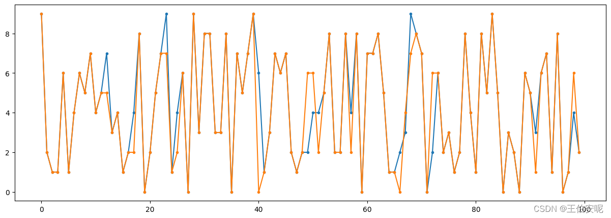
# 选取前 100 个数据进行绘制

plt.figure(figsize=(15,5))
plt.plot(data[:100],marker=".")
plt.show()

# 计算准确值和均方差
print(accuracy_score(result,y_test))
print(mean_squared_error(result,y_test))

"""
accuracy_score : 0.8412
mean_squared_error : 1.9939
"""

结果

 student-mat：G3为期末成绩

数据引用：

百度网盘 请输入提取码百度网盘为您提供文件的网络备份、同步和分享服务。空间大、速度快、安全稳固，支持教育网加速，支持手机端。注册使用百度网盘即可享受免费存储空间https://pan.baidu.com/s/1kYY1UyLh-MoASh6KWg_uJA?pwd=1111

 代码实现

import pandas as pd
import numpy as np
from sklearn.metrics import accuracy_score
from sklearn.linear_model import LogisticRegression
from sklearn.model_selection import train_test_split

# sep=";" 以;分割数据
data = pd.read_csv("student-mat.csv",sep=";")

# 创建一个新列 满足条件值为1否则为0
data["Degree"] = np.where(data["G3"].astype(int) >= 13, "1", "0")

# 选用5个变量作为X
X = data[["studytime","absences","G1","G2","G3"]].astype(int)
y = data['Degree'].values[:,np.newaxis].astype(int)

# 分割数据
X_train,X_test,y_train,y_test = train_test_split(X, y, test_size=0.1)

# 模型创建
model = LogisticRegression()
model.fit(X_train,y_train)

result = model.predict(X_test)

# 对模型进行评分
score = accuracy_score(result, y_test)

print(score)
# 1 数据简单 拟合较好

print(model.coef_)
# [[-0.02347521  0.05153924  0.19581741  0.82197572  3.49628117]]
# 影响因素 值越大 影响越大

index = ["Bad","Good"]

result_obj = [index[x] for x in result]
y_test_obj = [index[x] for x in y_test.reshape(-1)]

obj_data = pd.DataFrame({"Prediction":result_obj,"Actual":y_test_obj})
print(obj_data)

"""

Prediction	Actual
0	Good	Good
1	Bad	    Bad
2	Bad	    Bad
3	Bad	    Bad
4	Bad	    Bad
"""