卷积神经网络CNN

卷积神经网络是深度学习在计算机视觉领域的突破性成果。在计算机视觉领域，往往输入图像都很大，若使用全连接网络，计算代价较高。图像也很难保留原有的特征，导致图像处理的准确率不高卷积神经网络（Convolutional Neural Network）是含有卷积层的神经网络。卷积层的作用就是用来自动学习、提取图像的特征CNN网络主要有三部分构成：卷积层、池化层和全连接层构成，其中卷积层负责提取图像中的局部

GG_Bond18

1243人浏览 · 2025-02-14 00:32:29

GG_Bond18 · 2025-02-14 00:32:29 发布

一、CNN概述

卷积神经网络是深度学习在计算机视觉领域的突破性成果。在计算机视觉领域，往往输入图像都很大，若使用全连接网络，计算代价较高。图像也很难保留原有的特征，导致图像处理的准确率不高

卷积神经网络（Convolutional Neural Network）是含有卷积层的神经网络。卷积层的作用就是用来自动学习、提取图像的特征

CNN网络主要有三部分构成：卷积层、池化层和全连接层构成，其中卷积层负责提取图像中的局部特征；池化层用来大幅降低参数量级(降维)；全连接层用来输出想要的结果

二、图像基础知识

图像是由像素点组成的，每个像素点的值范围为[0, 255]，像素值越大意味着较亮。一张 200x200 的图像，则是由 40000 个像素点组成，若每个像素点都是 0，意味着这是一张全黑的图像

彩色图一般都是多通道的图像，所谓多通道可以理解为图像由多个不同的图像层叠加而成。平常的彩色图像一般都是由 RGB 三个通道组成的，还有一些图像具有 RGBA 四个通道，最后一个通道为透明通道，该值越小，则图像越透明

import numpy as np
import matplotlib.pyplot as plt

def test01():
    # 构建200 * 200, 像素值全为0的图像
    image = np.zeros([200, 200])
    plt.imshow(image, cmap='gray', vmin=0, vmax=255)
    plt.show()
    # 构建200 * 200, 像素值全为255的图像
    image = np.full([200, 200], 255)
    plt.imshow(image, cmap='gray', vmin=0, vmax=255)
    plt.show()

def test02():
    image = plt.imread('data/彩色图片.png')
    print(image.shape)
    # (640, 640, 4) 图像为 RGBA 四通道
    # 修改数据的维度, 将通道维度放在第一位
    image = np.transpose(image, [2, 0, 1])
    # 打印所有通道
    for channel in image:
        print(channel)
        plt.imshow(channel)
        plt.show()
    # 修改透明度
    image[3] = 0.05
    image = np.transpose(image, [1, 2, 0])
    plt.imshow(image)
    plt.show()

if __name__ == "__main__":
    test01()
    test02()

三、卷积层

3.1 卷积的计算

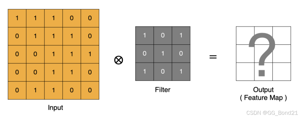
input 表示输入的图像
filter 表示卷积核, 也叫做滤波器
input 经过 filter 的得到输出为最右侧的图像，即特征图

卷积运算本质上就是在滤波器和输入数据的局部区域间做点积

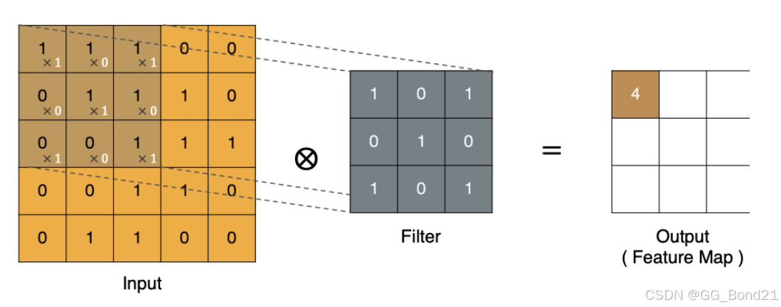
左上角的点计算方法：

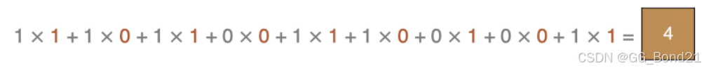
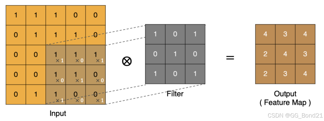
按照上面的计算方法可以得到最终的特征图为：

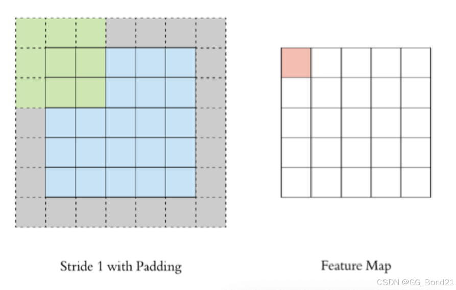
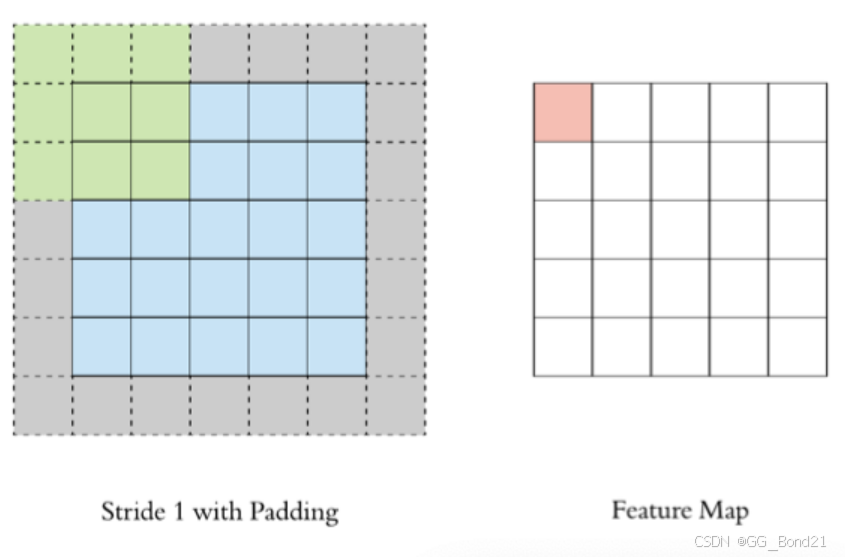
3.2 Padding

通过上面的卷积计算过程，最终的特征图会比原始图像小很多，若想要保持经过卷积后的图像大小不变，可以在原图周围添加 padding 再进行卷积来实现

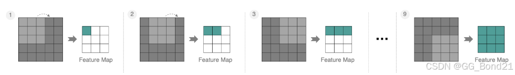
3.3 Stride

按照步长为1来移动卷积核，计算特征图如下所示：

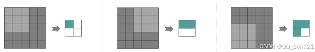
若将 Stride 增大为2，也是可以提取特征图的，如下图所示：

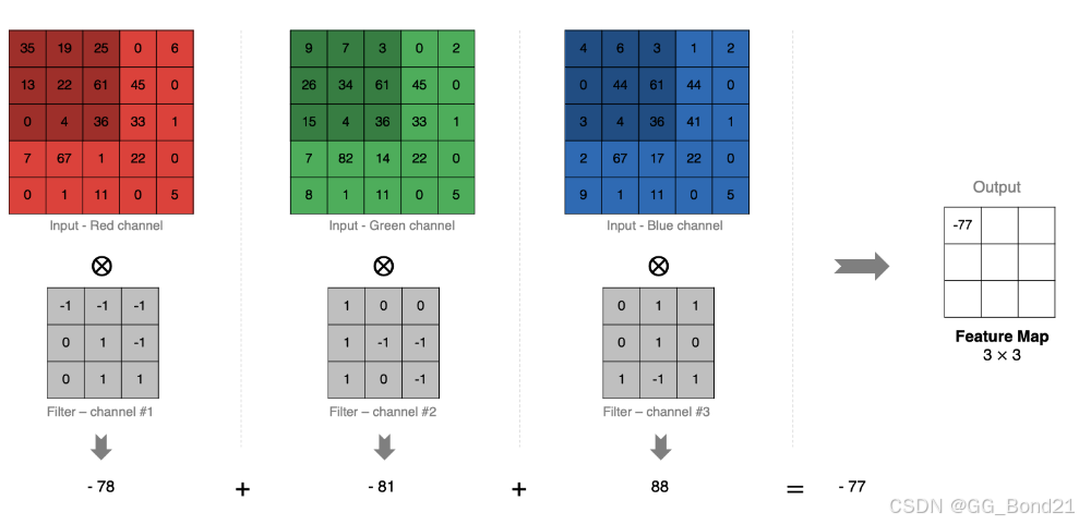
3.4 多通道卷积计算

实际中的图像都是多个通道组成的

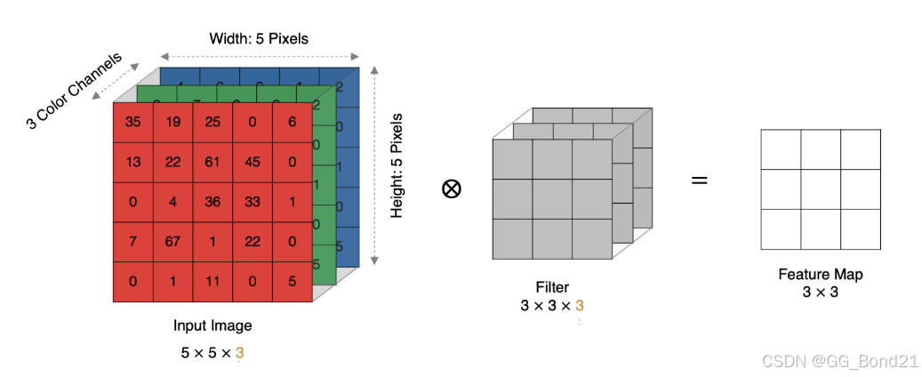
计算方法如下：

当输入有多个通道(Channel)，如 RGB 三个通道，此时要求卷积核需要拥有相同的通道数
每个卷积核通道与对应的输入图像的各个通道进行卷积
将每个通道的卷积结果按位相加得到最终的特征图

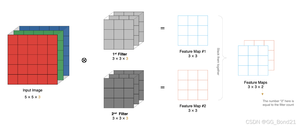
3.5 多卷积核卷积计算

实际对图像进行特征提取时，需要使用多个卷积核进行特征提取。可以理解为从不同到的视角、不同的角度对图像特征进行提取

3.6 特征图大小计算

输出特征图的大小与以下参数息息相关:

size：卷积核大小，一般会选择为奇数，如：1*1，3*3，5*5*
Padding：零填充的方式
Stride：步长

那计算方法如下图所示:

输入图像大小：W * W
卷积核大小: F * F
Stride：S
Padding：P
输出图像大小：N x N

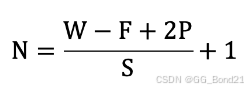
样例

图像大小：5 * 5
卷积核大小：3 * 3
Stride：1
Padding：1
(5 - 3 + 2) / 1 + 1 = 5，即得到的特征图大小为：5 * 5

3.7 Pytorch 卷积层API

import torch
import torch.nn as nn
import matplotlib.pyplot as plt

def show(image):
    plt.imshow(image)
    plt.axis('off')
    plt.show()

# 单个多通道卷积核
def test01():
    # 读取图片, 形状(640, 640, 4) HWC
    image = plt.imread('data/彩色图片.png')
    show(image)
    # 构建卷积层
    conv = nn.Conv2d(in_channels=4, out_channels=1, kernel_size=3, stride=1, padding=1)
    # 卷积层对输入数据的形状有要求,(batch_size, channel, height, weight)
    image = torch.tensor(image).permute(2, 0, 1)
    image = image.unsqueeze(0)
    print(image.shape)
    # 输入
    output_image = conv(image)
    print(output_image.shape)
    # 调整形状为正常图像形状
    output_image = output_image.squeeze(0).permute(1, 2, 0)
    show(output_image.detach().numpy())

# 多个多通道卷积核
def test02():
    # 读取图片, 形状(640, 640, 4) HWC
    image = plt.imread('data/彩色图片.png')
    show(image)
    # 构建卷积层
    # 由于out_channels为3, 相当于有3个4通道卷积核
    conv = nn.Conv2d(in_channels=4, out_channels=3, kernel_size=3, stride=1, padding=1)
    # 卷积层对输入数据的形状有要求,(batch_size, channel, height, weight)
    image = torch.tensor(image).permute(2, 0, 1)
    image = image.unsqueeze(0)
    # 输入
    output_image = conv(image)
    print(output_image.shape)
    # 调整形状为正常图像形状
    output_image = output_image.squeeze(0).permute(1, 2, 0)
    print(output_image.shape)
    # 打印三个特征图
    # 每组卷积核的参数不同, 在与输入图像进行卷积运算时会提取出不同的特征信息
    show(output_image[:, :, 0].unsqueeze(2).detach().numpy())
    show(output_image[:, :, 1].unsqueeze(2).detach().numpy())
    show(output_image[:, :, 2].unsqueeze(2).detach().numpy())

if __name__ == "__main__":
    test01()
    test02()

四、池化层

池化层 (Pooling) 降低维度，缩减模型大小，提高计算速度。主要对卷积层学习到的特征图进行下采样（SubSampling）处理

池化层主要有两种：最大池化、平均池化

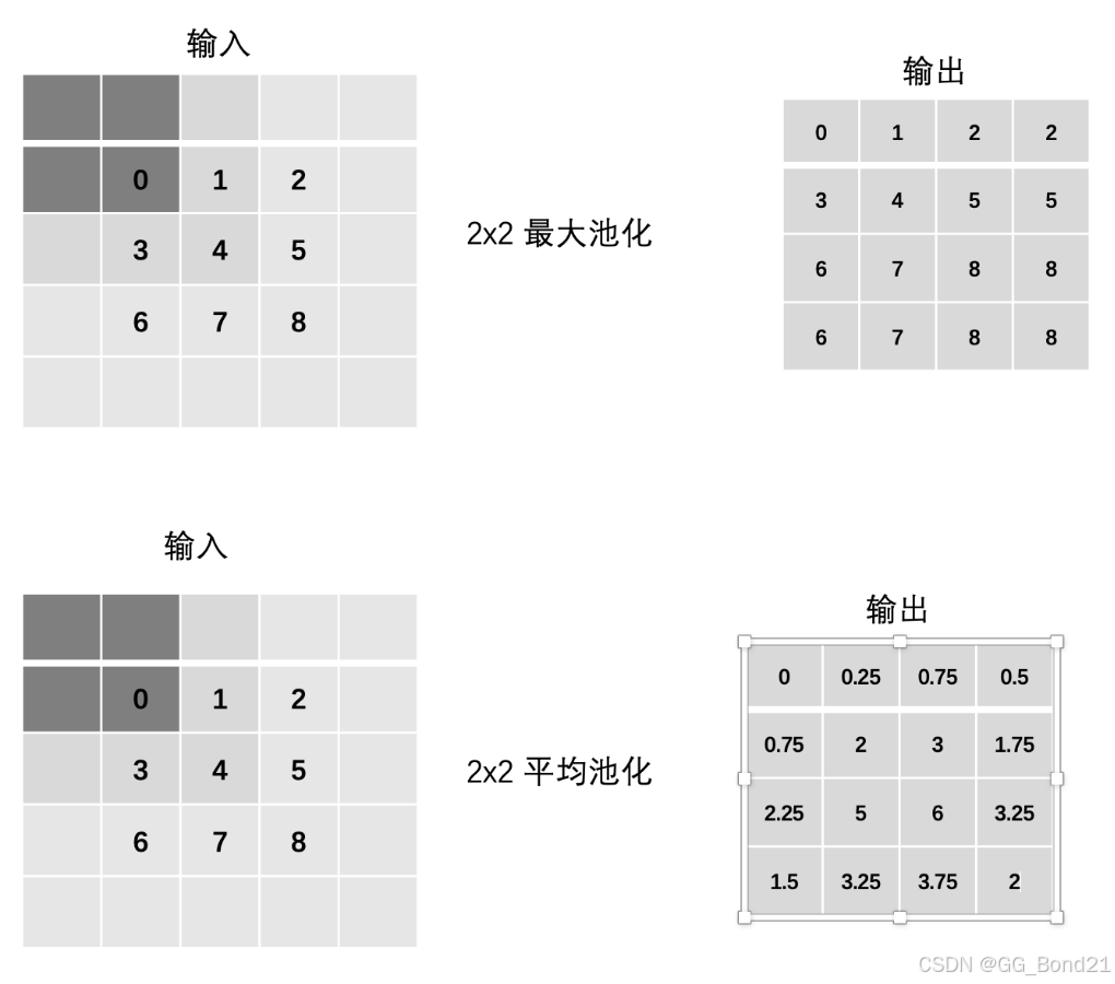
4.1 池化计算

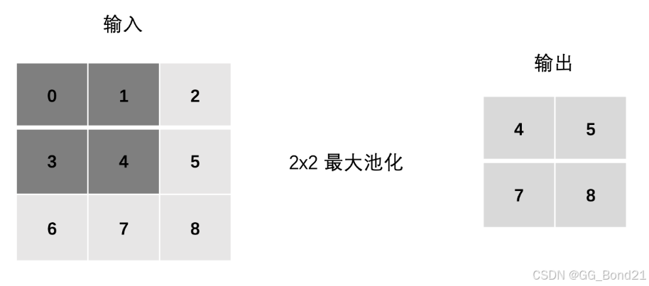
最大池化：

max(0，1，3，4)
max(1，2，4，5)
max(3，4，6，7)
max(4，5，7，8)

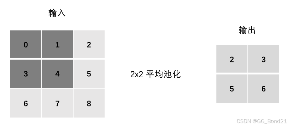
平均池化：

mean(0，1，3，4)
mean(1，2，4，5)
mean(3，4，6，7)
mean(4，5，7，8)

4.2 Stride

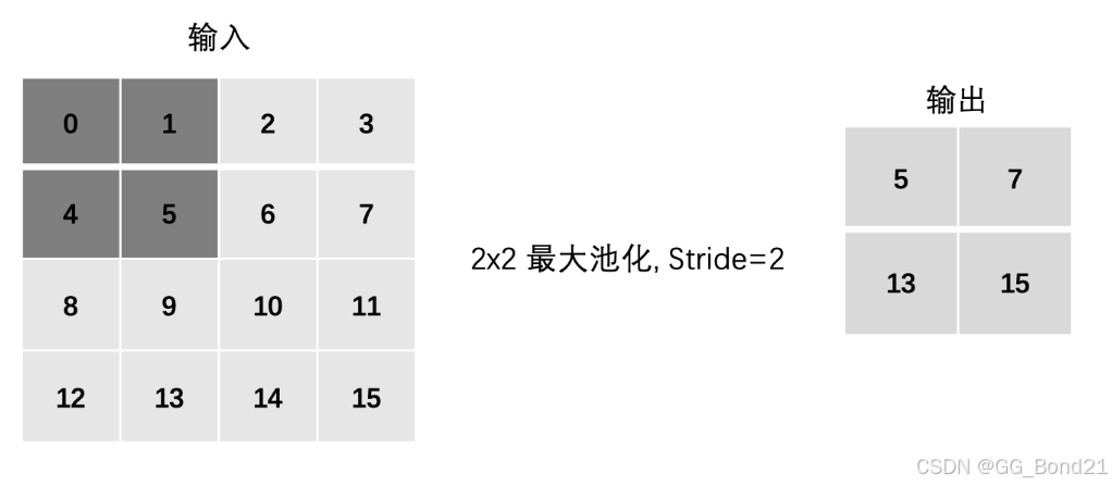
最大池化：

max(0，1，4，5)
max(2，3，6，7)
max(8，9，12，13)
max(10，11，14，15)

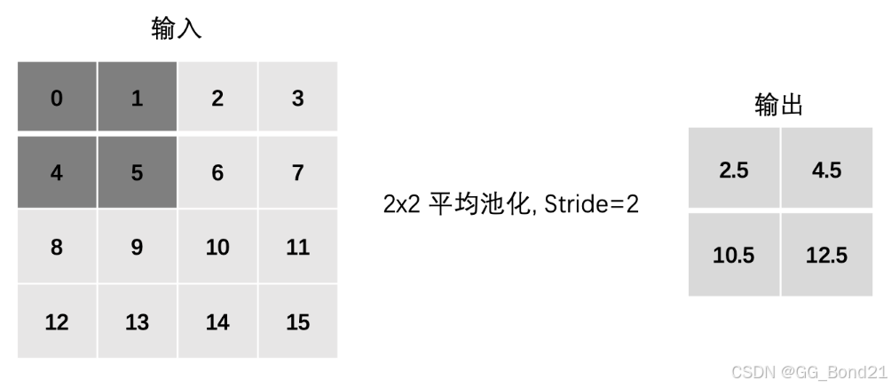
平均池化：

mean(0，1，4，5)
mean(2，3，6，7)
mean(8，9，12，13)
mean(10，11，14，15)

4.3 Padding

最大池化：

max(0，0，0，0)
max(0，0，0，1)
max(0，0，1，2)
max(0，0，2，0)
... 以此类推

平均池化：

mean(0，0，0，0)
mean(0，0，0，1)
mean(0，0，1，2)
mean(0，0，2，0)
... 以此类推

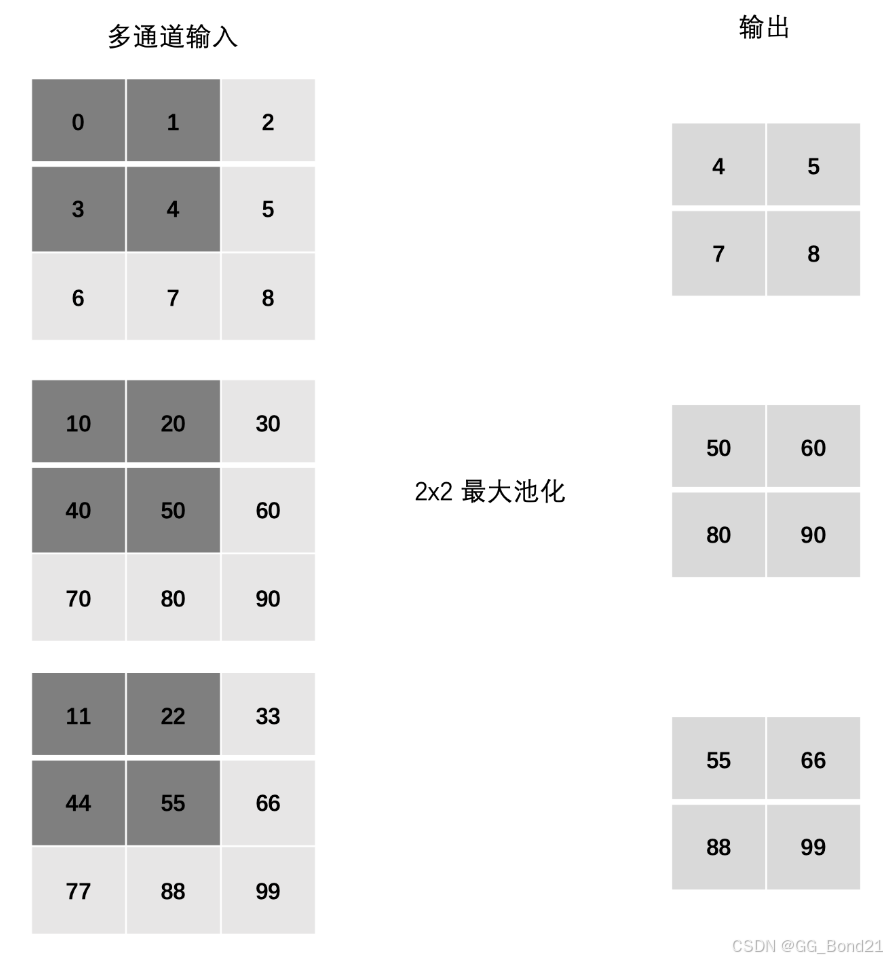
4.4 多通道池化计算

在处理多通道输入数据时，池化层对每个输入通道分别池化，而不是像卷积层那样将各个通道的输入相加。这意味着池化层的输出和输入的通道数是相等

即：卷积会改变通道数，池化不会改变通道数

4.5 Pytorch 池化层API

import torch
import torch.nn as nn

# 基本使用
def test01():
    inputs = torch.tensor([[0, 1, 2], [3, 4, 5], [6, 7, 8]]).float()
    inputs = inputs.unsqueeze(0).unsqueeze(0)
    # (1,1,3,3)
    print(inputs.shape)

    # 最大池化, 输入形状(batch_size, channel, height, weight)
    polling = nn.MaxPool2d(kernel_size=2, stride=1, padding=0)
    output = polling(inputs)
    print(output)
    # 平均池化
    polling = nn.AvgPool2d(kernel_size=2, stride=1, padding=0)
    output = polling(inputs)
    print(output)

# stride
def test02():
    inputs = torch.tensor([[0, 1, 2, 3], [4, 5, 6, 7], [8, 9, 10, 11], [12, 13, 14, 15]]).float()
    inputs = inputs.unsqueeze(0).unsqueeze(0)
    # 最大池化, 输入形状(batch_size, channel, height, weight)
    polling = nn.MaxPool2d(kernel_size=2, stride=2, padding=0)
    output = polling(inputs)
    print(output)
    # 平均池化
    polling = nn.AvgPool2d(kernel_size=2, stride=2, padding=0)
    output = polling(inputs)
    print(output)

# padding
def test03():
    inputs = torch.tensor([[0, 1, 2], [3, 4, 5], [6, 7, 8]]).float()
    inputs = inputs.unsqueeze(0).unsqueeze(0)
    # 最大池化, 输入形状(batch_size, channel, height, weight)
    polling = nn.MaxPool2d(kernel_size=2, stride=1, padding=1)
    output = polling(inputs)
    print(output)
    # 平均池化
    polling = nn.AvgPool2d(kernel_size=2, stride=1, padding=1)
    output = polling(inputs)
    print(output)

# 多通道池化
def test04():
    inputs = torch.tensor([[[0, 1, 2], [3, 4, 5], [6, 7, 8]],
                           [[10, 20, 30], [40, 50, 60], [70, 80, 90]],
                           [[11, 22, 33], [44, 55, 66], [77, 88, 99]]]).float()
    inputs.unsqueeze(0)
    # 最大池化, 输入形状(batch_size, channel, height, weight)
    polling = nn.MaxPool2d(kernel_size=2, stride=1, padding=0)
    output = polling(inputs)
    print(output)
    # 平均池化
    polling = nn.AvgPool2d(kernel_size=2, stride=1, padding=0)
    output = polling(inputs)
    print(output)

if __name__ == "__main__":
    # test01()
    # test02()
    # test03()
    test04()

技术共进，成长同行——讯飞AI开发者社区

更多推荐

2025 年 8 月科技前沿观察与未来展望

讯飞AI开发者社区

vLLM监控指标可视化------

浪潮信息KOS是浪潮信息基于Linux Kernel、OpenAnolis等开源技术自主研发的一款服务器操作系统，支持x86、ARM等主流架构处理器，性能和稳定性居于行业领先地位，具备成熟的 CentOS 迁移和替换能力，可满足云计算、大数据、分布式存储、人工智能、边缘计算等应用场景需求。详细介绍见官网链接id=12126vLLM是一种用于大规模语言模型（LLM）推理的框架，旨在提高模型的吞吐量和