该项目是复现的一篇论文的实验：

项目视频讲解：

机器学习国际原油价格预测-lstm原油价格预测-完整代码可直接运行-核心论文复现_哔哩哔哩_bilibili

项目运行结果：

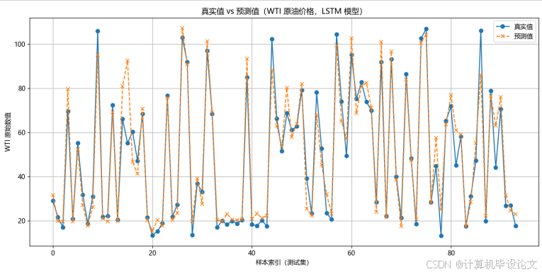
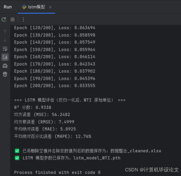
lstm实验结果：

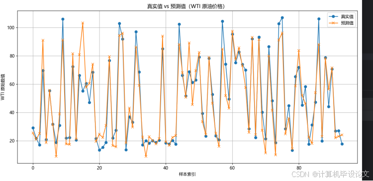
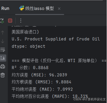
机器学习实验结果：

论文代码：

#!/usr/bin/env python3
# -*- coding: utf-8 -*-

"""
基于 LSTM 的回归示例（取代线性回归），并可视化真实值 vs 预测值（WTI 原油价格）

依赖：
  pip install pandas numpy matplotlib scikit-learn torch joblib
"""

import pandas as pd
import numpy as np
import matplotlib.pyplot as plt
import matplotlib
from sklearn.preprocessing import StandardScaler
from sklearn.metrics import (
    mean_squared_error, r2_score, mean_absolute_error, mean_absolute_percentage_error
)
from sklearn.model_selection import train_test_split
import torch
import torch.nn as nn
from torch.utils.data import Dataset, DataLoader
import joblib

# ================================
# 一、让 matplotlib 能正确显示中文
# ================================
plt.rcParams['font.family'] = 'Microsoft YaHei'   # Windows 下常见的中文字体
plt.rcParams['axes.unicode_minus'] = False        # 解决负号显示为方块的问题

# ================================
# Step 1：读取数据，删除空值与非数值列
# ================================
df = pd.read_excel('数据整合.xlsx')

print("=== 原始数据前 5 行 ===")
print(df.head(5))
print("\n=== 原始列名 ===")
print(df.columns.tolist())

df.dropna(inplace=True)
df = df.drop(columns=['observation_date'])  # 删除非数值列

print("\n=== 删除 observation_date 之后的列名 ===")
print(df.columns.tolist())
print("\n=== 各列数据类型 ===")
print(df.dtypes)

# ================================
# Step 2：标准化所有数值列
# ================================
scaler = StandardScaler()
df_scaled = pd.DataFrame(scaler.fit_transform(df), columns=df.columns)

# ================================
# Step 3：准备训练与测试数据（用于 LSTM）
# ================================
target_column = "WTI"
X = df_scaled.drop(columns=[target_column]).values  # shape=(n_samples, n_features)
y = df_scaled[target_column].values                  # shape=(n_samples,)

# 划分训练集与测试集
X_train, X_test, y_train, y_test = train_test_split(
    X, y, test_size=0.2, random_state=42, shuffle=True
)

# 将特征 reshape 为 LSTM 输入格式： (batch_size, seq_len, input_size)
# 这里把每条记录的各特征当做时间步，将 input_size 设为 1
n_features = X_train.shape[1]
input_size = 1
seq_len = n_features

X_train_seq = X_train.reshape(-1, seq_len, input_size)
X_test_seq  = X_test.reshape(-1, seq_len, input_size)

# ================================
# Step 4：定义 PyTorch Dataset
# ================================
class WTI_Dataset(Dataset):
    def __init__(self, X_seq, y_vals):
        self.X_seq = torch.from_numpy(X_seq).float()
        self.y_vals = torch.from_numpy(y_vals).float().unsqueeze(1)  # (N,1)
    def __len__(self):
        return self.X_seq.size(0)
    def __getitem__(self, idx):
        return self.X_seq[idx], self.y_vals[idx]

train_dataset = WTI_Dataset(X_train_seq, y_train)
test_dataset  = WTI_Dataset(X_test_seq,  y_test)

batch_size = 32
train_loader = DataLoader(train_dataset, batch_size=batch_size, shuffle=True)
test_loader  = DataLoader(test_dataset,  batch_size=batch_size, shuffle=False)

# ================================
# Step 5：定义 LSTM 回归模型
# ================================
class LSTMRegressor(nn.Module):
    def __init__(self, input_size, hidden_size=64, num_layers=1):
        super(LSTMRegressor, self).__init__()
        self.hidden_size = hidden_size
        self.num_layers = num_layers
        # 单向 LSTM
        self.lstm = nn.LSTM(
            input_size=input_size,
            hidden_size=hidden_size,
            num_layers=num_layers,
            batch_first=True,
            bidirectional=False
        )
        # 最后一层隐藏状态送到全连接层
        self.fc = nn.Linear(hidden_size, 1)

    def forward(self, x):
        # x: (batch_size, seq_len, input_size)
        batch_size = x.size(0)
        h0 = torch.zeros(self.num_layers, batch_size, self.hidden_size).to(x.device)
        c0 = torch.zeros(self.num_layers, batch_size, self.hidden_size).to(x.device)
        out, (hn, cn) = self.lstm(x, (h0, c0))
        # out: (batch_size, seq_len, hidden_size)
        # hn: (num_layers, batch_size, hidden_size)
        last_hidden = hn[-1]  # (batch_size, hidden_size)
        out = self.fc(last_hidden)  # (batch_size, 1)
        return out

# ================================
# Step 6：模型训练
# ================================
device = torch.device("cuda" if torch.cuda.is_available() else "cpu")
model = LSTMRegressor(input_size=input_size, hidden_size=64, num_layers=1).to(device)
criterion = nn.MSELoss()
optimizer = torch.optim.Adam(model.parameters(), lr=1e-3)

epochs = 200
model.train()
for epoch in range(1, epochs + 1):
    epoch_loss = 0.0
    for X_batch, y_batch in train_loader:
        X_batch = X_batch.to(device)
        y_batch = y_batch.to(device)
        optimizer.zero_grad()
        outputs = model(X_batch)  # (batch_size,1)
        loss = criterion(outputs, y_batch)
        loss.backward()
        optimizer.step()
        epoch_loss += loss.item() * X_batch.size(0)
    epoch_loss /= len(train_dataset)
    if epoch % 10 == 0 or epoch == 1:
        print(f"Epoch [{epoch}/{epochs}], Loss: {epoch_loss:.6f}")

# ================================
# Step 7：在测试集上预测
# ================================
model.eval()
y_pred_scaled = []
y_true_scaled = []
with torch.no_grad():
    for X_batch, y_batch in test_loader:
        X_batch = X_batch.to(device)
        preds = model(X_batch)  # (batch_size,1)
        y_pred_scaled.append(preds.cpu().numpy())
        y_true_scaled.append(y_batch.cpu().numpy())

y_pred_scaled = np.vstack(y_pred_scaled).flatten()  # (n_test,)
y_true_scaled = np.vstack(y_true_scaled).flatten()  # (n_test,)

# ================================
# Step 8：反归一化 —— 将 y_test、y_pred 还原到原始 WTI 数值
# ================================
target_index = df.columns.get_loc(target_column)
target_mean = scaler.mean_[target_index]
target_std  = np.sqrt(scaler.var_[target_index])

y_test_original = y_true_scaled * target_std + target_mean
y_pred_original = y_pred_scaled * target_std + target_mean

# ================================
# Step 9：计算多种回归评价指标（基于原始数值）
# ================================
mse = mean_squared_error(y_test_original, y_pred_original)
rmse = np.sqrt(mse)
mae = mean_absolute_error(y_test_original, y_pred_original)
mape = mean_absolute_percentage_error(y_test_original, y_pred_original)
r2 = r2_score(y_test_original, y_pred_original)

print("\n=== LSTM 模型评估（反归一化后，WTI 原始单位） ===")
print(f"R² 分数: {r2:.4f}")
print(f"均方误差 (MSE): {mse:.4f}")
print(f"均方根误差 (RMSE): {rmse:.4f}")
print(f"平均绝对误差 (MAE): {mae:.4f}")
print(f"平均绝对百分比误差 (MAPE): {mape * 100:.2f}%")

# ================================
# Step 10：可视化 —— 反归一化后的真实值 vs 预测值
# ================================
plt.figure(figsize=(12, 6))
plt.plot(y_test_original, label="真实值", marker='o', linestyle='-')
plt.plot(y_pred_original, label="预测值", marker='x', linestyle='--')
plt.title("真实值 vs 预测值（WTI 原油价格，LSTM 模型）")
plt.xlabel("样本索引（测试集）")
plt.ylabel("WTI 原始数值")
plt.legend()
plt.grid(True)
plt.tight_layout()
plt.show()

# ================================
# Step 11：保存“清洗后”的数据和模型
# ================================
df.to_excel("数据整合_cleaned.xlsx", index=False)
print("\n✅ 已将删除空值并去除非数值列后的数据保存为：数据整合_cleaned.xlsx")

joblib.dump(model.state_dict(), "lstm_model_WTI.pth")
print("✅ LSTM 模型参数已保存为：lstm_model_WTI.pth")

import pandas as pd
import numpy as np
import matplotlib.pyplot as plt
import matplotlib
from sklearn.preprocessing import StandardScaler
from sklearn.linear_model import LinearRegression
from sklearn.metrics import (
    mean_squared_error, r2_score, mean_absolute_error, mean_absolute_percentage_error
)
from sklearn.model_selection import train_test_split
import joblib

# ================================
# 一、让 matplotlib 能正确显示中文
# ================================
plt.rcParams['font.family'] = 'Microsoft YaHei'   # Windows 下常见的中文字体
plt.rcParams['axes.unicode_minus'] = False        # 解决负号显示为方块的问题

# ================================
# Step 1：读取数据，删除空值与非数值列
# ================================
# 1.1 读取 Excel
df = pd.read_excel('数据整合.xlsx')

# 1.2 打印前几行和列名，方便检查
print("=== 原始数据前 5 行 ===")
print(df.head(5))
print("\n=== 原始列名 ===")
print(df.columns.tolist())

# 1.3 删除含有 NaN 的整行
df.dropna(inplace=True)

# 1.4 删除 “observation_date” 列（非数值），以及其他非目标数值列
#     假设我们要用除 “observation_date” 之外的所有列来预测 WTI，
#     那么先把它删掉。其余列中如果有非数值，也需要剔除；此处示例中只删除 observation_date。
df = df.drop(columns=['observation_date'])

# 1.5 再次检查：确保 WTI 在列名里且都是数值类型
print("\n=== 删除 observation_date 之后的列名 ===")
print(df.columns.tolist())
print("\n=== 各列数据类型 ===")
print(df.dtypes)

# 如果有其它非数值列（dtype 为 object），请在这里一并 drop。例如：
# df = df.drop(columns=['某个非数值列名'])

# ================================
# Step 2：标准化所有数值列
# ================================
scaler = StandardScaler()

# 关键：给 DataFrame 指定 columns=df.columns，保持列名一致
df_scaled = pd.DataFrame(scaler.fit_transform(df), columns=df.columns)

# ================================
# Step 3：构建线性回归模型并训练、预测
# ================================
# 3.1 设置目标列
target_column = "WTI"

# 3.2 划分特征 X 与目标 y
X = df_scaled.drop(columns=[target_column])
y = df_scaled[target_column]

# 3.3 切分训练集与测试集
X_train, X_test, y_train, y_test = train_test_split(
    X, y, test_size=0.2, random_state=42
)

# 3.4 训练线性回归模型
model = LinearRegression()
model.fit(X_train, y_train)

# 3.5 用测试集做预测（得到的是标准化后的 y_pred）
y_pred_scaled = model.predict(X_test)

# ================================
# Step 4：反归一化 —— 将 y_test、y_pred 还原到“原始 WTI 数值”
# ================================
# 4.1 找到目标列在原始 df 中的下标
target_index = df.columns.get_loc(target_column)

# 4.2 从 scaler 中取出对应的 mean 和 std
target_mean = scaler.mean_[target_index]
target_std = np.sqrt(scaler.var_[target_index])  # 或者直接用 scaler.scale_[target_index]

# 4.3 反归一化
y_test_original = y_test * target_std + target_mean
y_pred_original = y_pred_scaled * target_std + target_mean

# ================================
# Step 5：计算多种回归评价指标（基于原始数值）
# ================================
mse = mean_squared_error(y_test_original, y_pred_original)
rmse = np.sqrt(mse)
mae = mean_absolute_error(y_test_original, y_pred_original)
mape = mean_absolute_percentage_error(y_test_original, y_pred_original)
r2 = r2_score(y_test_original, y_pred_original)

print("\n=== 模型评估（反归一化后，WTI 原始单位） ===")
print(f"R² 分数: {r2:.4f}")
print(f"均方误差 (MSE): {mse:.4f}")
print(f"均方根误差 (RMSE): {rmse:.4f}")
print(f"平均绝对误差 (MAE): {mae:.4f}")
print(f"平均绝对百分比误差 (MAPE): {mape * 100:.2f}%")

# ================================
# Step 6：可视化 —— 反归一化后的真实值 vs 预测值
# ================================
plt.figure(figsize=(12, 6))
plt.plot(y_test_original.values, label="真实值", marker='o')
plt.plot(y_pred_original,       label="预测值", marker='x')
plt.title("真实值 vs 预测值（WTI 原油价格）")
plt.xlabel("样本索引")
plt.ylabel("WTI 原始数值")
plt.legend()
plt.grid(True)
plt.tight_layout()
plt.show()

# ================================
# Step 7：保存“清洗后”的数据和模型
# ================================
# 7.1 保存清洗后的原始 DataFrame
df.to_excel("数据整合_cleaned.xlsx", index=False)
print("\n✅ 已将删除空值并去除非数值列后的数据保存为：数据整合_cleaned.xlsx")

# 7.2 保存训练好的模型
joblib.dump(model, "linear_model_WTI.pkl")
print("✅ 线性回归模型已保存为：linear_model_WTI.pkl")

完整代码数据：https://download.csdn.net/download/weixin_55771290/90966512