
深度学习训练营-基于DCGAN的图像生成实战-Task2-DCGAN生成手写数字图片实战-20240506
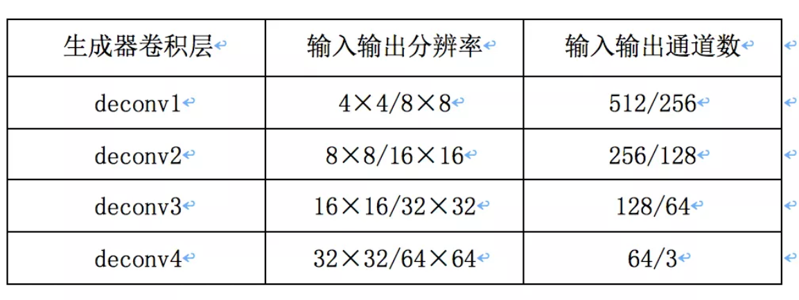
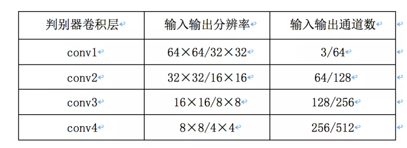
DCGAN 是第⼀个全卷积 GAN,⿇雀虽⼩,五脏俱全,最适合新⼈实践。DCGAN的⽣成器和判别器都采⽤了4层的⽹络结构。⽣成器⽹络结构如上图所⽰,输⼊为1×100的向量,然后经过⼀个全连接层学习,reshape为 4×4×1024的张量,再经过4个上采样的反卷积⽹络层,⽣成64×64的图,各层的配置如下:判别器输⼊64×64⼤⼩的图,经过4次卷积,分辨率降低为4×4的⼤⼩,每⼀个卷积层的配置如下
文章目录
本任务将在 MNIST 数据集上完成一个 DCGAN 的项目。
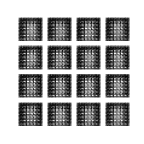
下方动画展示了当训练了 50 个epoch (全部数据集迭代50次) 时生成器所生成的一系列图片。图片从随机噪声开始,随着时间的推移越来越像手写数字。
接下来我们进⾏实践,选择 PyTorch 框架,下⾯详解具体的⼯程代码,主要包括:
- 运行环境与数据集准备
- 创建模型
- 定义损失函数与优化器
- 训练模型
- 可视化
原理简介
DCGAN 是第⼀个全卷积 GAN,⿇雀虽⼩,五脏俱全,最适合新⼈实践。
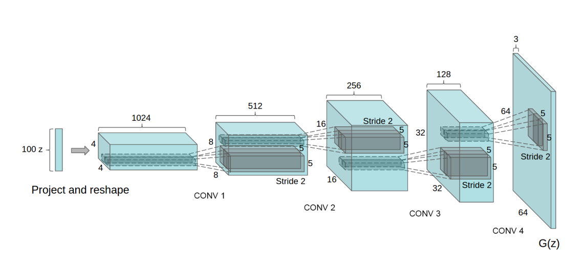
DCGAN的⽣成器和判别器都采⽤了4层的⽹络结构。⽣成器⽹络结构如上图所⽰,输⼊为1×100的向量,然后经过⼀个全连接层学习,reshape为 4×4×1024的张量,再经过4个上采样的反卷积⽹络层,⽣成64×64的图,各层的配置如下:
判别器输⼊64×64⼤⼩的图,经过4次卷积,分辨率降低为4×4的⼤⼩,每⼀个卷积层的配置如下:
接下来我们进⾏实践,选择 PyTorch 框架,下⾯详解具体的⼯程代码,主要包括:
- 运行环境与数据集准备
- 创建模型
- 定义损失函数与优化器
- 训练模型
- 可视化
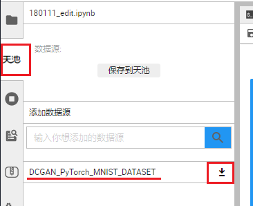
运行环境与数据集准备
- 在加载该 NoteBook 文件时,会自动加载数据集至
./download/DCGAN_PyTorch_MNIST_DATASET文件夹下。若没有自动加载数据集,则需要手动加载,手动加载方式如下:
点击本页面左方 天池 按钮(需要在 CPU 环境下),点击 DCGAN_PyTorch_MNIST_DATASET 旁边的下载按钮,就会自动加载数据集了!
import time
import torch
import torch.nn as nn
from torch.utils.data import DataLoader
from torchvision import utils, datasets, transforms
import matplotlib.pyplot as plt
import matplotlib.animation as animation
from IPython.display import HTML
1. 加载和准备数据集
本项目使用 MNIST 数据集来训练生成器和判别器。生成器将生成类似于 MNIST 数据集的手写数字。 首先加载数据集,并设置初始参数。
在加载该 NoteBook 文件时,会自动加载数据集自
DCGAN_PyTorch_MNIST_DATASET文件夹下
dataroot = "./DCGAN_PyTorch_MNIST_DATASET/"  # 数据集所在的路径,我们已经事先下载下来了
workers = 10  # 数据加载时的进程数
batch_size = 100  # 生成器输入的大小

image_size = 64  # 训练图像的大小
nc = 1  # 训练图像的通道数,彩色图像的话就是 3
nz = 100  # 输入是100 维的随机噪声 z,看作是 100 个 channel,每个特征图宽高是 1*1
ngf = 64  # 生成器中特征图的大小,
ndf = 64  # 判别器中特征图的大小
num_epochs = 10  # 训练的轮次
lr = 0.0002  # 学习率大小
beta1 = 0.5  # Adam 优化器的参数
ngpu = 1  # 可用 GPU  的个数,0 代表使用 CPU

# 训练集加载并进行归一化等操作
train_data = datasets.MNIST(
    root=dataroot,
    train=True,
    transform=transforms.Compose([
        transforms.Resize(image_size),
        transforms.ToTensor(),
        transforms.Normalize((0.5, ), (0.5, ))
    ]),
    download=True  # 从互联网下载,如果已经下载的话,就直接使用
)

# 测试集加载并进行归一化等操作
test_data = datasets.MNIST(root=dataroot,
                           train=False,
                           transform=transforms.Compose([
                               transforms.Resize(image_size),
                               transforms.ToTensor(),
                               transforms.Normalize((0.5, ), (0.5, ))
                           ]))

# 把 MNIST 的训练集和测试集都用来做训练
dataset = train_data + test_data
print(f'Total Size of Dataset: {len(dataset)}')

# 数据加载器,训练过程中不断产生数据
dataloader = DataLoader(dataset=dataset,
                        batch_size=batch_size,
                        shuffle=True,
                        num_workers=workers)

# 看是否存在可用的 GPU
device = torch.device('cuda:0' if (
    torch.cuda.is_available() and ngpu > 0) else 'cpu')

# 权重初始化函数
def weights_init(m):
    classname = m.__class__.__name__
    if classname.find('Conv') != -1:
        nn.init.normal_(m.weight.data, 0.0, 0.02)
    elif classname.find('BatchNorm') != -1:
        nn.init.normal_(m.weight.data, 1.0, 0.02)
        nn.init.constant_(m.bias.data, 0)
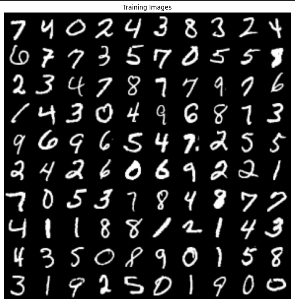
以下的代码用做读取部分数据集进行展示,看看我们原始输入的数据是怎么样的。
inputs = next(iter(dataloader))[0]
plt.figure(figsize=(10, 10))
plt.title("Training Images")
plt.axis('off')
inputs = utils.make_grid(inputs[:100] * 0.5 + 0.5, nrow=10)
plt.imshow(inputs.permute(1, 2, 0))
创建模型
1. 生成器
生成器使用 torch.nn.ConvTranspose2d (上采样)层来从种子(随机噪声)中产生图片。以一个使用该种子作为输入的 Dense 层开始,然后多次上采样直到达到所期望的 64x64x1 的图片尺寸。注意除了输出层使用 tanh 之外,其他每层均使用 torch.nn.functional.relu 作为激活函数。
下面定义一个生成器的类,读者可以依照生成器网络配置理解以下代码
class Generator(nn.Module):
    def __init__(self, ngpu):
        super(Generator, self).__init__()
        self.ngpu = ngpu
        self.main = nn.Sequential(
            # input is Z, going into a convolution
            nn.ConvTranspose2d(in_channels=nz,
                               out_channels=ngf * 8,
                               kernel_size=4,
                               stride=1,
                               padding=0,
                               bias=False),
            nn.BatchNorm2d(ngf * 8),
            nn.ReLU(True),
            # 当前特征图大小  (ngf*8) x 4 x 4
            nn.ConvTranspose2d(ngf * 8, ngf * 4, 4, 2, 1, bias=False),
            nn.BatchNorm2d(ngf * 4),
            nn.ReLU(True),
            # 当前特征图大小 (ngf*4) x 8 x 8
            nn.ConvTranspose2d(ngf * 4, ngf * 2, 4, 2, 1, bias=False),
            nn.BatchNorm2d(ngf * 2),
            nn.ReLU(True),
            # 当前特征图大小 (ngf*2) x 16 x 16
            nn.ConvTranspose2d(ngf * 2, ngf, 4, 2, 1, bias=False),
            nn.BatchNorm2d(ngf),
            nn.ReLU(True),
            # 当前特征图大小 (ngf) x 32 x 32
            nn.ConvTranspose2d(ngf, nc, 4, 2, 1, bias=False),
            nn.Tanh()
            # 当前特征图大小 (nc) x 64 x 64
        )

    def forward(self, input):
        return self.main(input)
2. 判别器
判别器是一个基于 CNN 的图片分类器。
class Discriminator(nn.Module):
    def __init__(self, ngpu):
        super(Discriminator, self).__init__()
        self.ngpu = ngpu
        self.main = nn.Sequential(
            # 输入 (nc) x 64 x 64
            nn.Conv2d(nc, ndf, 4, 2, 1, bias=False),
            nn.LeakyReLU(0.2, inplace=True),
            # 当前特征图大小 (ndf) x 32 x 32
            nn.Conv2d(ndf, ndf * 2, 4, 2, 1, bias=False),
            nn.BatchNorm2d(ndf * 2),
            nn.LeakyReLU(0.2, inplace=True),
            # 当前特征图大小 (ndf*2) x 16 x 16
            nn.Conv2d(ndf * 2, ndf * 4, 4, 2, 1, bias=False),
            nn.BatchNorm2d(ndf * 4),
            nn.LeakyReLU(0.2, inplace=True),
            # 当前特征图大小 (ndf*4) x 8 x 8
            nn.Conv2d(ndf * 4, ndf * 8, 4, 2, 1, bias=False),
            nn.BatchNorm2d(ndf * 8),
            nn.LeakyReLU(0.2, inplace=True),
            # 当前特征图大小 (ndf*8) x 4 x 4
            nn.Conv2d(ndf * 8, 1, 4, 1, 0, bias=False),
            # 当前特征图大小 (1) x 1 x 1
            nn.Sigmoid())

    def forward(self, input):
        return self.main(input)
3. 生成器与判别器初始化
# 创建一个生成器对象
netG = Generator(ngpu).to(device)
# 多卡并行,如果有多卡的话
if device.type == 'cuda' and ngpu > 1:
    netG = nn.DataParallel(netG, list(range(ngpu)))

# 初始化权重  其中,mean=0, stdev=0.2.
netG.apply(weights_init)

# 创建一个判别器对象
netD = Discriminator(ngpu).to(device)
# 多卡并行,如果有多卡的话
if device.type == 'cuda' and ngpu > 1:
    netD = nn.DataParallel(netD, list(range(ngpu)))

# 初始化权重  其中,mean=0, stdev=0.2.
netD.apply(weights_init)
定义损失函数和优化器
为两个模型定义损失函数和优化器。
criterion = nn.BCELoss()  # 定义损失函数

# 创建一批潜在向量,我们将使用它们来可视化生成器的生成过程
fixed_noise = torch.randn(100, nz, 1, 1, device=device)

real_label = 1.  # “真”标签
fake_label = 0.  # “假”标签

# 为生成器和判别器定义优化器
optimizerG = torch.optim.Adam(netG.parameters(), lr=lr, betas=(beta1, 0.999))
optimizerD = torch.optim.Adam(netD.parameters(), lr=lr, betas=(beta1, 0.999))
训练阶段
DCGAN 的训练过程如下:
1、首先固定 Generator,训练 Discriminator
- 输入:真实数据 x x x,Generator 生成的数据 G ( x ) G(x) G(x)
- 输出:二分类概率
从噪声分布中随机采样噪声 z z z,经过 Generator 生成 G ( z ) G(z) G(z)。G(z)和 x 输入到 Discriminator 得到 D ( x ) D(x) D(x) 和 D ( G ( z ) ) D(G(z)) D(G(z)),损失函数为
1 m ∑ i = 1 m [ log D ( x ( i ) ) + log ( 1 − D ( G ( z ( i ) ) ) ) ] \frac{1}{m} \sum_{i=1}^{m}\left[\log D\left(\boldsymbol{x}^{(i)}\right)+\log \left(1-D\left(G\left(\boldsymbol{z}^{(i)}\right)\right)\right)\right] m1i=1∑m[logD(x(i))+log(1−D(G(z(i))))]
这里是最大化损失函数,因此使用梯度上升法更新参数。
2、固定 Discriminator,训练 Generator。
- 输入:随机噪声 z z z
- 输出:分类概率 D ( G ( z ) ) D(G(z)) D(G(z)),目的是使 D ( G ( z ) ) = 1 D(G(z))=1 D(G(z))=1
从噪声分布中重新随机采样噪声 z z z,经过 Generator 生成 G ( z ) G(z) G(z)。 G ( z ) G(z) G(z) 输入到 Discriminator 得到 D ( G ( z ) ) D(G(z)) D(G(z)),损失函数为
1 m ∑ i = 1 m log ( 1 − D ( G ( z ( i ) ) ) ) \frac{1}{m} \sum_{i=1}^{m} \log \left(1-D\left(G\left(z^{(i)}\right)\right)\right) m1i=1∑mlog(1−D(G(z(i))))
这里是最小化损失函数,使用梯度下降法更新参数。
# 定义一些变量,用来存储每轮的相关值
img_list = []
G_losses = []
D_losses = []
D_x_list = []
D_z_list = []
loss_tep = 10

print("Starting Training Loop...")
# 迭代
for epoch in range(num_epochs):
    beg_time = time.time()
    # 数据加载器读取数据
    for i, data in enumerate(dataloader):
        ############################
        # (1) Update D network: maximize log(D(x)) + log(1 - D(G(z)))
        ###########################
        # 用所有的真数据进行训练
        netD.zero_grad()
        # Format batch
        real_cpu = data[0].to(device)
        b_size = real_cpu.size(0)
        label = torch.full((b_size, ),
                           real_label,
                           dtype=torch.float,
                           device=device)

        # 判别器推理
        output = netD(real_cpu).view(-1)

        # Calculate loss on all-real batch
        # 计算所有真标签的损失函数
        errD_real = criterion(output, label)
        # Calculate gradients for D in backward pass
        errD_real.backward()
        D_x = output.mean().item()

        # 生成假数据并进行训练
        noise = torch.randn(b_size, nz, 1, 1, device=device)

        # 用生成器生成假图像
        fake = netG(noise)
        label.fill_(fake_label)
        # Classify all fake batch with D
        output = netD(fake.detach()).view(-1)
        # 计算判别器在假数据上的损失
        errD_fake = criterion(output, label)
        errD_fake.backward()
        D_G_z1 = output.mean().item()
        # Add the gradients from the all-real and all-fake batches
        errD = errD_real + errD_fake
        # Update D
        optimizerD.step()

        ############################
        # (2) Update G network: maximize log(D(G(z)))
        ###########################
        netG.zero_grad()
        label.fill_(real_label)  # fake labels are real for generator cost
        # Since we just updated D, perform another forward pass of all-fake batch through D
        output = netD(fake).view(-1)
        # Calculate G's loss based on this output
        errG = criterion(output, label)
        # Calculate gradients for G
        errG.backward()
        D_G_z2 = output.mean().item()
        # Update G
        optimizerG.step()

        # Output training stats
        end_time = time.time()
        run_time = round(end_time - beg_time)
        print(f'Epoch: [{epoch+1:0>{len(str(num_epochs))}}/{num_epochs}]',
              f'Step: [{i+1:0>{len(str(len(dataloader)))}}/{len(dataloader)}]',
              f'Loss-D: {errD.item():.4f}',
              f'Loss-G: {errG.item():.4f}',
              f'D(x): {D_x:.4f}',
              f'D(G(z)): [{D_G_z1:.4f}/{D_G_z2:.4f}]',
              f'Time: {run_time}s',
              end='\r')

        # Save Losses for plotting later
        G_losses.append(errG.item())
        D_losses.append(errD.item())

        # Save D(X) and D(G(z)) for plotting later
        D_x_list.append(D_x)
        D_z_list.append(D_G_z2)

        # 保存最好的模型
        if errG < loss_tep:
            torch.save(netG.state_dict(), 'model.pt')
            temp = errG

    # Check how the generator is doing by saving G's output on fixed_noise
    with torch.no_grad():
        fake = netG(fixed_noise).detach().cpu()
    img_list.append(utils.make_grid(fake * 0.5 + 0.5, nrow=10))
    print()
模型训练完毕后,会保存成一个 model.pt 文件
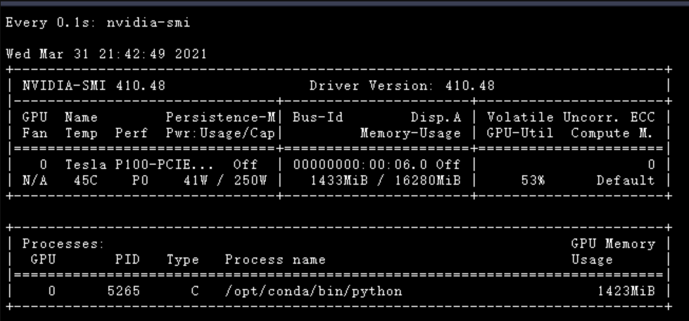
在运行过程中,可以打开终端,查看 GPU 运行情况

然后在终端运行以下命令!
watch -n 0.1 nvidia-smi
可视化
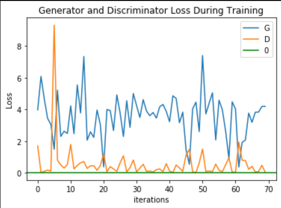
1. 生成器与判别器损失函数曲线
plt.title("Generator and Discriminator Loss During Training")
plt.plot(G_losses[::100], label="G")
plt.plot(D_losses[::100], label="D")
plt.xlabel("iterations")
plt.ylabel("Loss")
plt.axhline(y=0, label="0", c="g")  # asymptote
plt.legend()
2. 训练过程展示
fig = plt.figure(figsize=(10, 10))
plt.axis("off")
ims = [[plt.imshow(item.permute(1, 2, 0), animated=True)] for item in img_list]
ani = animation.ArtistAnimation(fig,
                                ims,
                                interval=1000,
                                repeat_delay=1000,
                                blit=True)
HTML(ani.to_jshtml())
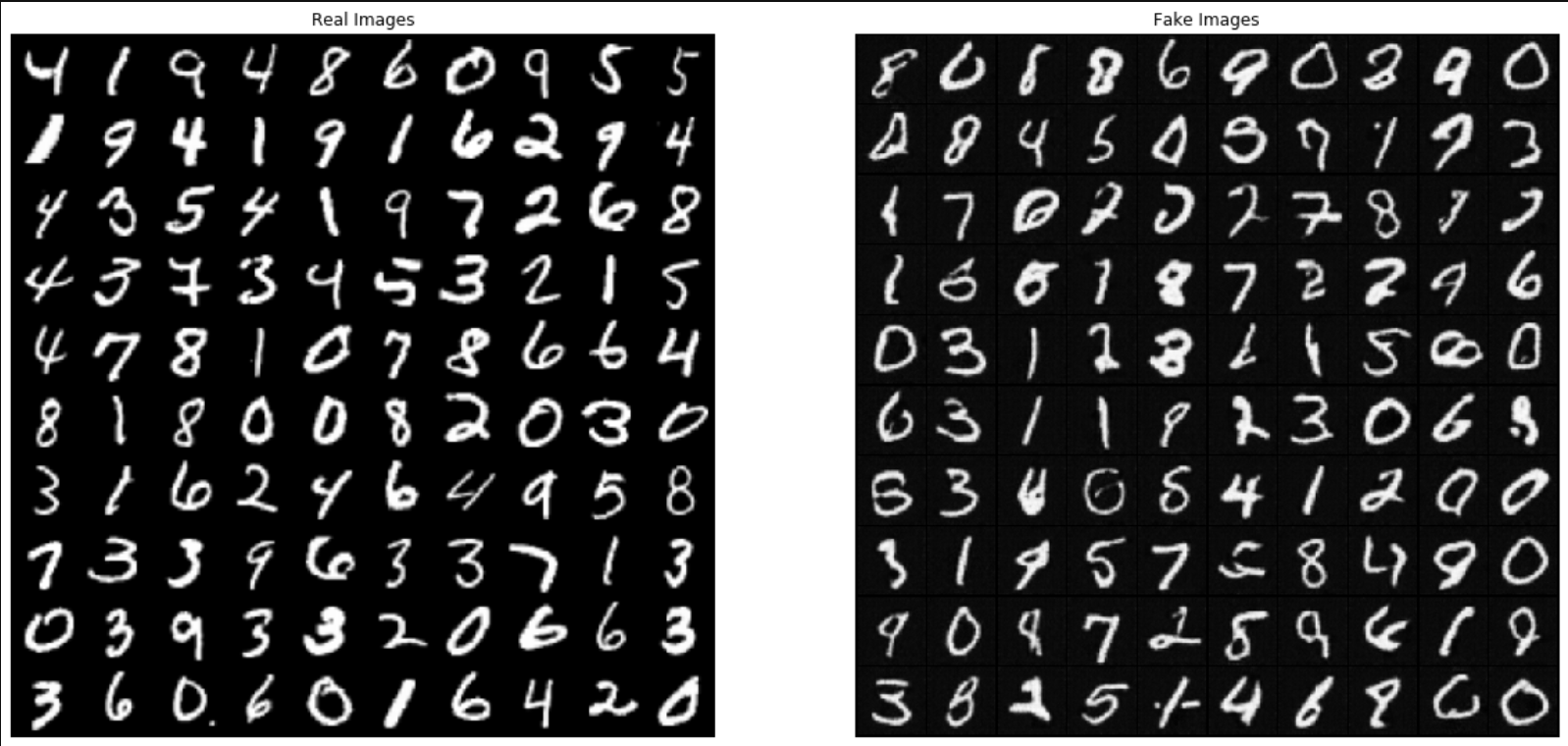
3. 真(训练集中的)——假(网络生成的)图片对比
# Size of the Figure
plt.figure(figsize=(20, 10))

# Plot the real images
plt.subplot(1, 2, 1)
plt.axis("off")
plt.title("Real Images")
real = next(iter(dataloader))
plt.imshow(
    utils.make_grid(real[0][:100] * 0.5 + 0.5, nrow=10).permute(1, 2, 0))

# Load the Best Generative Model
netG = Generator(0)
netG.load_state_dict(torch.load('model.pt', map_location=torch.device('cpu')))
netG.eval()

# Generate the Fake Images
with torch.no_grad():
    fake = netG(fixed_noise.cpu())

# Plot the fake images
plt.subplot(1, 2, 2)
plt.axis("off")
plt.title("Fake Images")
fake = utils.make_grid(fake * 0.5 + 0.5, nrow=10)
plt.imshow(fake.permute(1, 2, 0))

# Save the comparation result
plt.savefig('result.jpg', bbox_inches='tight')
参考来源

技术共进,成长同行——讯飞AI开发者社区
更多推荐

 0
0 0
0- 0


 已为社区贡献3条内容

所有评论(0)