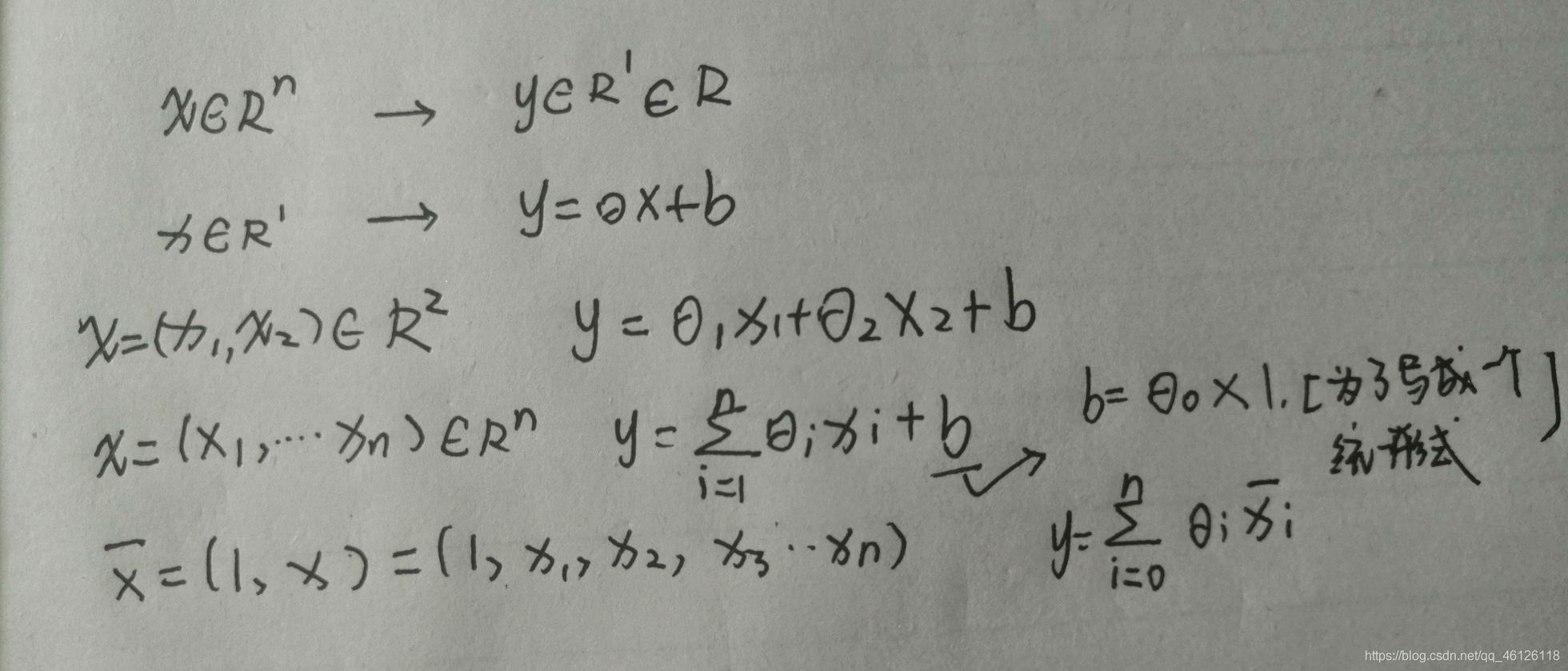
一.回顾线性回归知识点

二.作业实战

一.单变量的线性回归

【1】导入需要的包

import numpy as np
import pandas as pd
import matplotlib.pyplot as plt

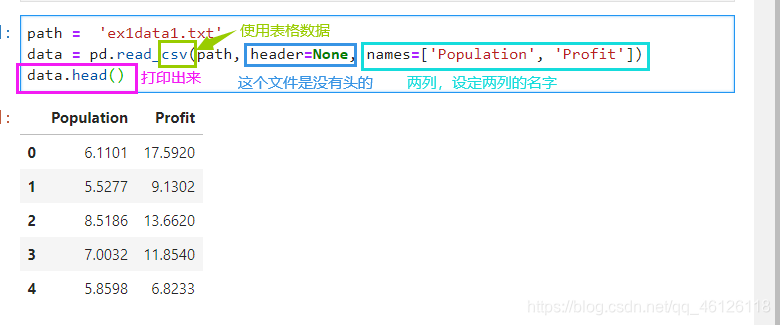
【2】导入数据集并查看

一定要把数据集和程序放在同一个文件夹里面，

path =  'ex1data1.txt'
data = pd.read_csv(path, header=None, names=['Population', 'Profit'])
data.head()

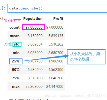
对于数值数据，结果的索引包括技术，平均值，标准差，最小值，最大值以及较低的百分位数和，默认情况下，较低百分位数为25，较高爆分位数为75,50百分位数和中位数相同

data.describe()data.describe()

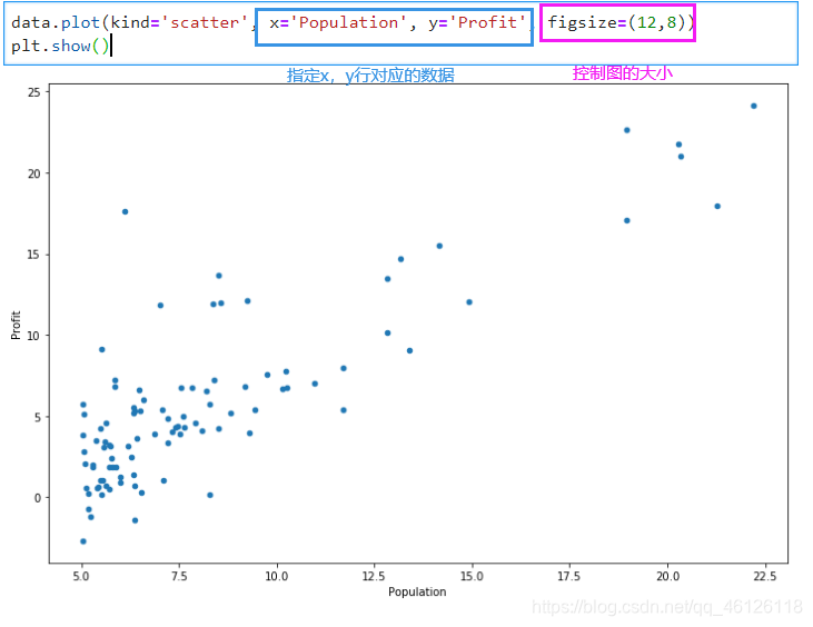
数据可视化，绘制散点图

data.plot(kind='scatter', x='Population', y='Profit', figsize=(12,8))
plt.show()

【3】使用梯度下降

现在让我们使用梯度下降来实现线性回归，以最小化成本函数
首先，我们将创建一个以参数θ为特征函数的代价函数
$$J\left(\theta \right)=\frac{1}{2m}\sum _{i=1}^m{\left(h_{\theta }\left(x^{(i)}\right)-y^{(i)}\right)}^2$$
其中：$h_{\theta }\left(x\right)={\theta }^{T}X={\theta }_0{x}_0+{\theta }_1{x}_1+{\theta }_2{x}_2+...+{\theta }_n{x}_n$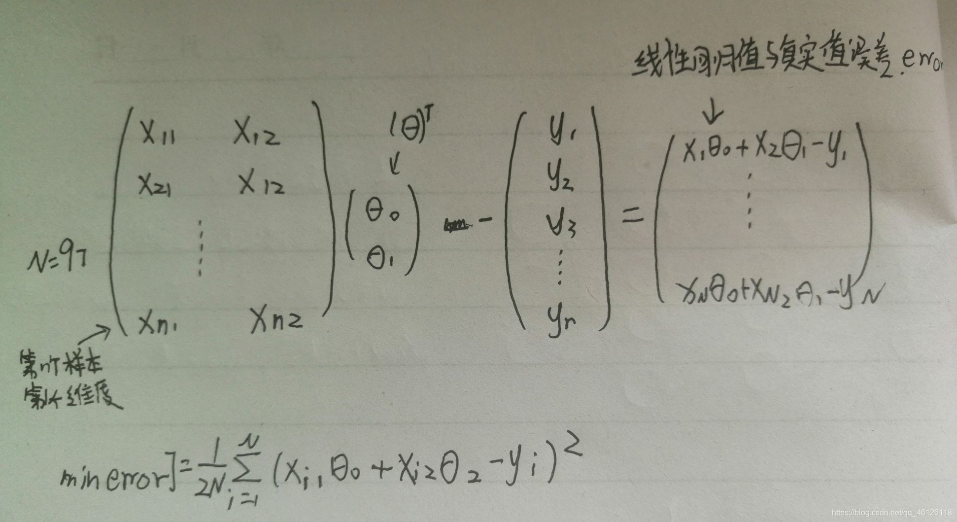

def computeCost(X, y, theta):
    inner = np.power(((X * theta.T) - y), 2)
    return np.sum(inner) / (2 * len(X))

np.power——就是如果后面跟一个矩阵，和数字，用逗号隔开，那么就把矩阵每一项（数字）方

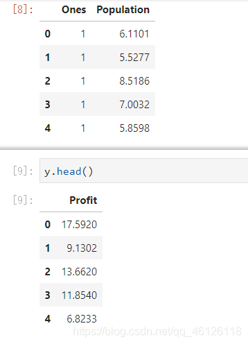
让我们在训练集中添加一列，以便我们可以使用向量化的解决方案来计算代价和梯度

data.insert(0, 'Ones', 1)

【4】变量初始化

# set X (training data) and y (target variable)
cols = data.shape[1]
X = data.iloc[:,0:cols-1]#X是所有行，去掉最后一列
y = data.iloc[:,cols-1:cols]#X是所有行，最后一列

观察下 X (训练集) and y (目标变量)是否正确.

X.head()#head()是观察前5行

代价函数是应该是numpy矩阵，所以我们需要转换X和Y，然后才能使用它们。 我们还需要初始化theta。

X = np.matrix(X.values)
y = np.matrix(y.values)
theta = np.matrix(np.array([0,0]))

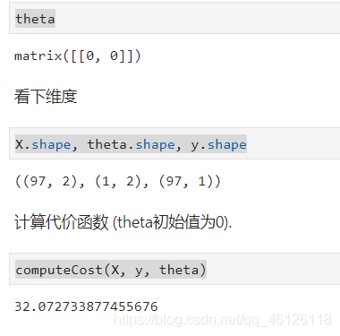
theta 是一个(1,2)矩阵

theta

matrix([[0, 0]])

看下维度

X.shape, theta.shape, y.shape

计算代价函数 (theta初始值为0).
调用这个函数输出

computeCost(X, y, theta)

【5】batch gradient decent（批量梯度下降）

$${\theta }_j:={\theta }_j-\alpha \frac{\partial }{\partial {\theta }_j}J\left(\theta \right)$$

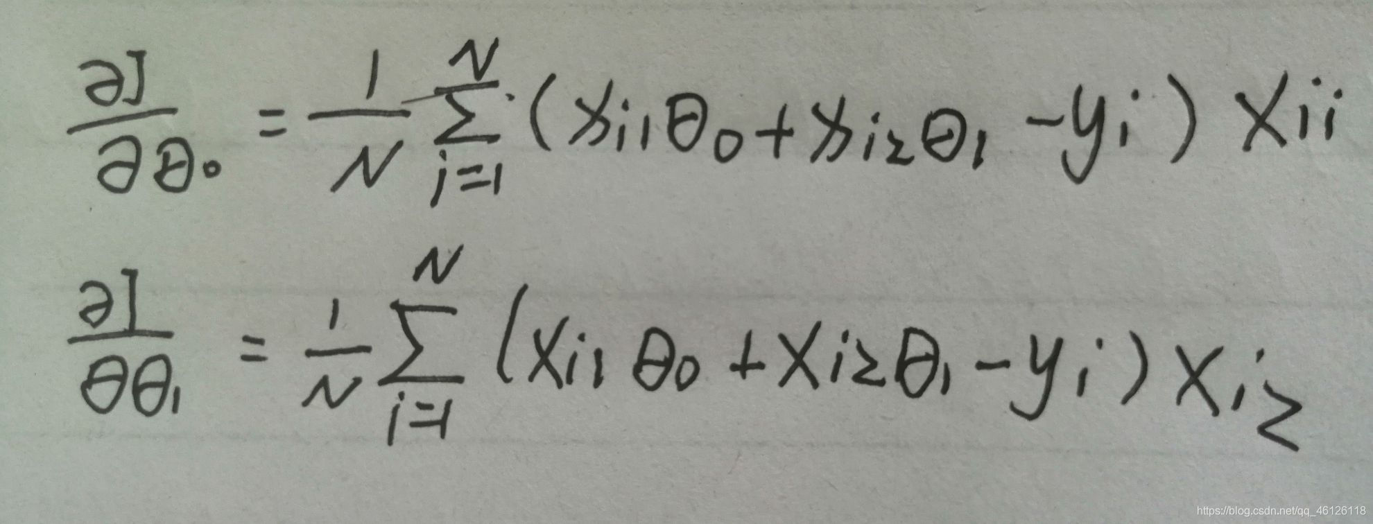
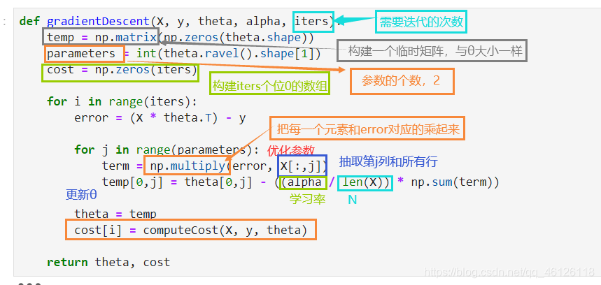
def gradientDescent(X, y, theta, alpha, iters):
    temp = np.matrix(np.zeros(theta.shape))
    parameters = int(theta.ravel().shape[1])
    cost = np.zeros(iters)
    
    for i in range(iters):
        error = (X * theta.T) - y
        
        for j in range(parameters):
            term = np.multiply(error, X[:,j])
            temp[0,j] = theta[0,j] - ((alpha / len(X)) * np.sum(term))
            
        theta = temp
        cost[i] = computeCost(X, y, theta)
        
    return theta, cost

初始化一些附加变量 - 学习速率α和要执行的迭代次数。

alpha = 0.01
iters = 1000

现在让我们运行梯度下降算法来将我们的参数θ适合于训练集。

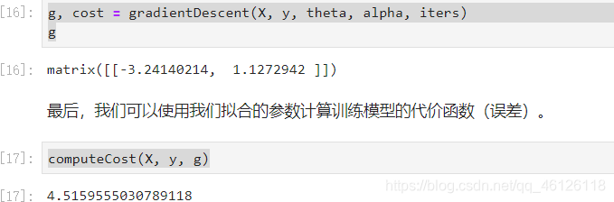
g, cost = gradientDescent(X, y, theta, alpha, iters)
g

最后，我们可以使用我们拟合的参数计算训练模型的代价函数（误差）

computeCost(X, y, g)

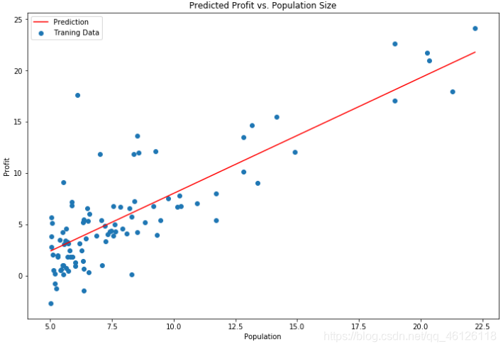
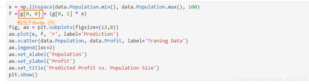
【6】绘制线性模型以及数据，直观地看出它的拟合

x = np.linspace(data.Population.min(), data.Population.max(), 100)
f = g[0, 0] + (g[0, 1] * x)

fig, ax = plt.subplots(figsize=(12,8))
ax.plot(x, f, 'r', label='Prediction')
ax.scatter(data.Population, data.Profit, label='Traning Data')
ax.legend(loc=2)
ax.set_xlabel('Population')
ax.set_ylabel('Profit')
ax.set_title('Predicted Profit vs. Population Size')
plt.show()

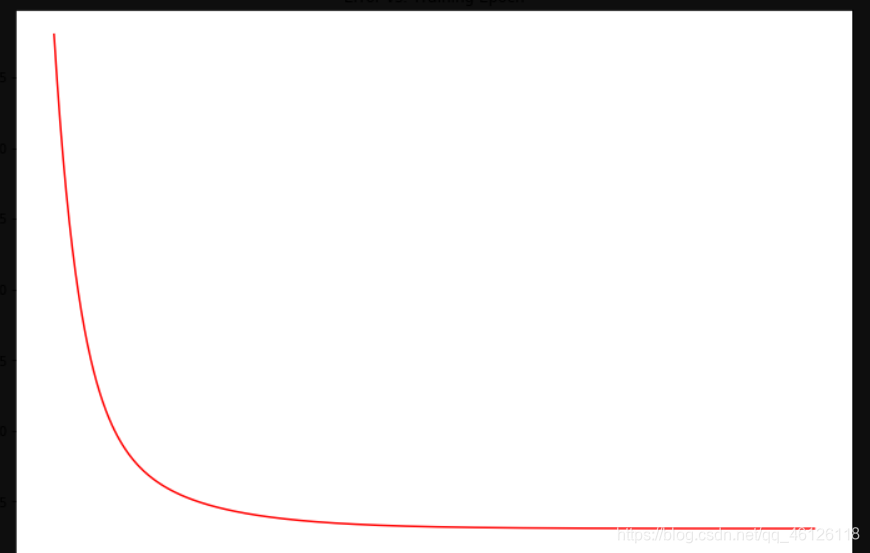
由于梯度方程式函数也在每个训练迭代中输出一个代价的向量，所以我们也可以绘制。 请注意，代价总是降低 - 这是凸优化问题的一个例子。

fig, ax = plt.subplots(figsize=(12,8))
ax.plot(np.arange(iters), cost, 'r')
ax.set_xlabel('Iterations')
ax.set_ylabel('Cost')
ax.set_title('Error vs. Training Epoch')
plt.show()

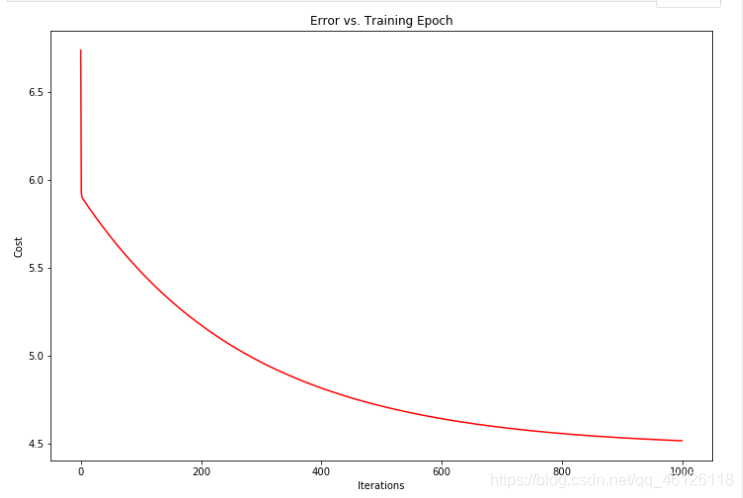
迭代次数越来越多，越来越收敛

二.多变量线性回归

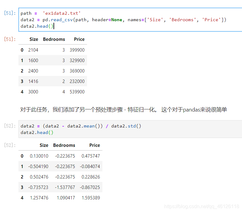
path =  'ex1data2.txt'
data2 = pd.read_csv(path, header=None, names=['Size', 'Bedrooms', 'Price'])
data2.head()

添加了另一个预处理步骤 - 特征归一化。

data2 = (data2 - data2.mean()) / data2.std()
data2.head()

现在我们重复第1部分的预处理步骤，并对新数据集运行线性回归程序

# add ones column
data2.insert(0, 'Ones', 1)

# set X (training data) and y (target variable)
cols = data2.shape[1]
X2 = data2.iloc[:,0:cols-1]
y2 = data2.iloc[:,cols-1:cols]

# convert to matrices and initialize theta
X2 = np.matrix(X2.values)
y2 = np.matrix(y2.values)
theta2 = np.matrix(np.array([0,0,0]))

# perform linear regression on the data set
g2, cost2 = gradientDescent(X2, y2, theta2, alpha, iters)

# get the cost (error) of the model
computeCost(X2, y2, g2)

0.13070336960771892

快速查看训练进程。

fig, ax = plt.subplots(figsize=(12,8))
ax.plot(np.arange(iters), cost2, 'r')
ax.set_xlabel('Iterations')
ax.set_ylabel('Cost')
ax.set_title('Error vs. Training Epoch')
plt.show()

scikit-learn model的预测表现

我们也可以使用scikit-learn的线性回归函数，而不是从头开始实现这些算法。 我们将scikit-learn的线性回归算法应用于第1部分的数据，并看看它的表现

from sklearn import linear_model
model = linear_model.LinearRegression()
model.fit(X, y)

LinearRegression(copy_X=True, fit_intercept=True, n_jobs=None, normalize=False)

x = np.array(X[:, 1].A1)
f = model.predict(X).flatten()

fig, ax = plt.subplots(figsize=(12,8))
ax.plot(x, f, 'r', label='Prediction')
ax.scatter(data.Population, data.Profit, label='Traning Data')
ax.legend(loc=2)
ax.set_xlabel('Population')
ax.set_ylabel('Profit')
ax.set_title('Predicted Profit vs. Population Size')
plt.show()

三. normal equation（正规方程）

正规方程是通过求解下面的方程来找出使得代价函数最小的参数的：$\frac{\partial }{\partial {\theta }_j}J\left({\theta }_j\right)=0$ 。
假设我们的训练集特征矩阵为 X（包含了$x_0=1$）并且我们的训练集结果为向量 y，则利用正规方程解出向量 $\theta ={\left(X^{T}X\right)}^{-1}{X}^{T}y$ 。
上标T代表矩阵转置，上标-1 代表矩阵的逆。设矩阵$A=X^{T}X$，则：${\left(X^{T}X\right)}^{-1}=A^{-1}$

梯度下降与正规方程的比较：

梯度下降：需要选择学习率α，需要多次迭代，当特征数量n大时也能较好适用，适用于各种类型的模型

正规方程：不需要选择学习率α，一次计算得出，需要计算${\left(X^{T}X\right)}^{-1}$，如果特征数量n较大则运算代价大，因为矩阵逆的计算时间复杂度为$O(n3)$，通常来说当$n$小于10000 时还是可以接受的，只适用于线性模型，不适合逻辑回归模型等其他模型

正规方程

def normalEqn(X, y):
    theta = np.linalg.inv(X.T@X)@X.T@y#X.T@X等价于X.T.dot(X)
    return theta

final_theta2=normalEqn(X, y)#感觉和批量梯度下降的theta的值有点差距

final_theta2

matrix([[-3.89578088],
[ 1.19303364]])
#梯度下降得到的结果是matrix([[-3.24140214, 1.1272942 ]])