
【AI核心能力】第6讲 从零手搓一个深度学习网络
解释了为什么需要深度学习,实现了激活函数、求拓扑序列、自动求导,手写了前后向传播和优化代码,得到一个一维深度学习网络,并给出了多维版本和二维版本的可视化结果。
第6讲 从零手搓一个深度学习网络
在之前的机器学习章节中,我们说到了为什么研究线性变化是必要的。但是在现实生活中,线性变化能拟合得事件是有限的,比如城市人口增长、区域病毒传染,往往会呈现一个S型曲线,这个现象主要归因于以下两点限制 (Constraints):
- 自然特性 Natural —— 病毒传染能力确实存在一上限
- 环境资源 Environment Resources —— 城市的资源有限
那么在数学上如何去刻画这种S型增长呢?
对比线性关系思考一下,这个我们要找的函数,似乎yt越大,则yt+1越小;同时又满足yt+1始终大于yt
yt+1∝ytyt+1∝(1−yt) y_{t+1}\propto y_t\\ y_{t+1}\propto (1-y_t) yt+1∝ytyt+1∝(1−yt)
所以在t时刻,这个函数满足
yt+1=yt(1−yt) y_{t+1}=y_t(1-y_t) yt+1=yt(1−yt)
即我们要找的函数的导数满足
f′(x)=f(x)(1−f(x)) f'(x) = f(x)(1-f(x)) f′(x)=f(x)(1−f(x))
这样的约束关系。
所以解这个微分方程得到
f(x)=11+e−x f(x)=\frac{1}{1+e^{-x}} f(x)=1+e−x1
这个函数就是激活函数 (activation function) —— sigmoid。
激活函数 Activation Function
import numpy as np

def sigmoid(x):
	return 1 / (1 + np.exp(-x))
sub_x = np.linspace(-10, 10)

import matplotlib.pyplot as plt

plt.plot(sub_x, sigmoid(sub_x))
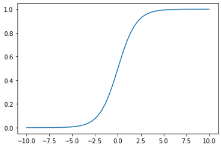
有了sigmoid函数,我们就可以用它来拟合上面提到的那些有限制条件的问题
import random

def random_linear(x):
	k, b = random.normalvariate(0, 1), random.normalvariate(0, 1)
	return k * x + b

for _ in range(5):
	plt.plot(sub_x, random_linear(sigmoid(random_linear(sub_x))))
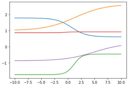
但是,现实生活中经常会存在更加复杂的函数,比如波浪型,那怎么办呢?
Complexity Functions Generated by Simple Functions
我们稍微改动一下代码,用index将sub_x分成两个数组,
index = np.random.choice(range(len(sub_x)))

y = np.concatenate((random_linear(sigmoid(random_linear(sub_x[:index]))), random_linear(sigmoid(random_linear(sub_x[index:])))))

plt.plot(sub_x, y)
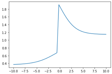
神奇的是,使用 一个线性函数 + 一个非线性函数 (激活函数sigmoid) 就可以生成很多复杂的函数。
原因是线性函数叠加线性函数只能生成线性结果,而激活函数的作用就是让我们的模型能够拟合非线性的关系,从而从理论上拟合出任意复杂的函数。
还记得我们之前在机器学习中讲到的loss函数吗?在现在的语境下就变成了
loss=1n∑(ytrue−y^)2=1n∑(ytrue−[k21e−(k1x+b1)+b2])2 loss=\frac{1}{n}\sum(y_{true}-\hat{y})^2=\frac{1}{n}\sum(y_{true}-[k_2\frac{1}{e^{-(k_1x+b1)}}+b2])^2 loss=n1∑(ytrue−y^)2=n1∑(ytrue−[k2e−(k1x+b1)1+b2])2
我们对loss求关于k1、k2、b1、b2的偏导
∇k1=∂loss∂k1∇k2=∂loss∂k2∇b1=∂loss∂b1∇b2=∂loss∂b2 \nabla k_1 = \frac{\partial loss}{\partial k_1}\\ \nabla k_2 = \frac{\partial loss}{\partial k_2}\\ \nabla b_1 = \frac{\partial loss}{\partial b_1}\\ \nabla b_2 = \frac{\partial loss}{\partial b_2}\\ ∇k1=∂k1∂loss∇k2=∂k2∂loss∇b1=∂b1∂loss∇b2=∂b2∂loss
然后
k1+=−∇k1αk2+=−∇k2αb1+=−∇b1αb2+=−∇b2α k_1+=-\nabla k_1\alpha\\ k_2+=-\nabla k_2\alpha\\ b_1+=-\nabla b_1\alpha\\ b_2+=-\nabla b_2\alpha\\ k1+=−∇k1αk2+=−∇k2αb1+=−∇b1αb2+=−∇b2α
来更新各参数。
可是我们发现,对于上面的loss函数很难求偏导。事实上,深度学习网络 (Deep Neural Network) 中一般包含着3个以上的线性函数和3个以上的非线性函数,求偏导的会极其复杂。
自动求导
无论是Pytorch还是TensorFlow,它们做的大部分工作就是自动求导。
我们把上面loss函数的结构拆一下
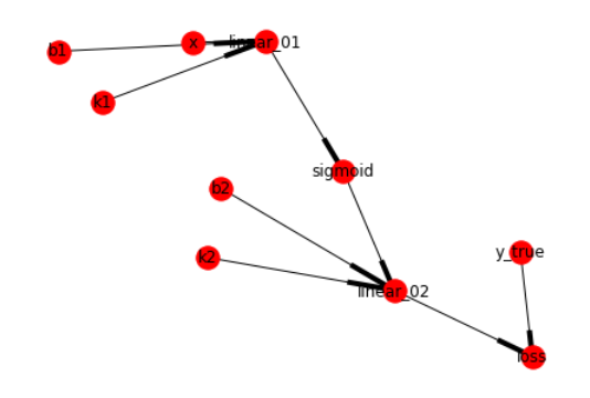
k1x+b1→linear_01linear_01→sigmoidsigmoid→linear_02linear_02 & ytrue→loss k_1x+b1\rightarrow linear\_01\\ linear\_01\rightarrow sigmoid\\ sigmoid\rightarrow linear\_02\\ linear\_02 \space \& \space y_{true}\rightarrow loss k1x+b1→linear_01linear_01→sigmoidsigmoid→linear_02linear_02 & ytrue→loss
可以发现,这种节点之间的连接关系很类似我们学过的一种数据结构 —— 图 (Graph)
所以,loss对k1求偏导的过程其实就是在图中找到这样一条从loss到k1的路径,也就是链式求导
∂loss∂k1=∂loss∂linear_02⋅∂linear_02∂sigmoid⋅∂sigmoid∂linear_01⋅∂linear_01∂k1 \frac{\partial loss}{\partial k_1} = \frac{\partial loss}{\partial linear\_02} \cdot \frac{\partial linear\_02}{\partial sigmoid} \cdot \frac{\partial sigmoid}{\partial linear\_01} \cdot \frac{\partial linear\_01}{\partial k_1} ∂k1∂loss=∂linear_02∂loss⋅∂sigmoid∂linear_02⋅∂linear_01∂sigmoid⋅∂k1∂linear_01
要找到这样一条路径,计算机必须知道节点的先后顺序,自然地想到我们需要对这些节点进行拓扑排序 (Topological Sort) —— {x, k1, b1, linear_01, sigmoid, k2, b2, linear_02, y_true, loss}。排序之后,我们就可以根据这个顺序来决定链式求导的先后了。
前后向传播原理 Feedforward & Feedbackward
前向传播和后向传播是深度学习的精髓,也是最重要和最难懂的部分。
为了方便理解,这里用代码演示一下
首先定义一个Node类。其子类Placeholder表示边缘节点 (无输入的,如x、k、b),Operator表示函数 (有输入的),它们在各自的前向传播和后向传播方法中会打印具体做了什么
class Node:
    def __init__(self, name, inputs=[]):
        self.name = name
        self.inputs = inputs
        self.outputs = []

        for node in self.inputs:
            node.outputs.append(self)

    def forward(self):
        print('Get self value'.format(self))

    def backward(self):
        pass

    def __repr__(self):
        return self.name


class Placeholder(Node):
    def __init__(self, name):
        Node.__init__(self, name=name)

    def forward(self):
        print('  Get my value from INITIAL')

    def backward(self):
        print('  I get my gradient from MEMORY directly')


class Operator(Node):
    def __init__(self, name, inputs=[]):
        Node.__init__(self, name=name, inputs=inputs)

    def forward(self):
        print('  Get my value by caculate: {}'.format(self.inputs))

    def backward(self):
        print('  Get Gradients ∂loss / ∂{} save to MEMORY'.format(self.inputs))
        if self.outputs:
            for n in self.inputs:
                print('    ==:> ∂loss / ∂{} = ∂loss / ∂{} * ∂{} / ∂{}'.format(n, self, self, n))
        else:  # Loss has no outputs
            print('    I am the final node')
接下来构建图
node_x = Placeholder('x')
node_k1 = Placeholder('k1')
node_b1 = Placeholder('b1')
node_linear01 = Operator('linear_01', inputs=[node_x, node_k1, node_b1])
node_sigmoid = Operator('sigmoid', inputs=[node_linear01])
node_k2 = Placeholder('k2')
node_b2 = Placeholder('b2')
node_linear02 = Operator('linear_02', inputs=[node_sigmoid, node_k2, node_b2])
node_y_true = Placeholder('y_true')
node_loss = Operator('loss', inputs=[node_y_true, node_linear02])
computer_graph = {
    node_k1: [node_linear01],
    node_b1: [node_linear01],
    node_x: [node_linear01],
    node_linear01: [node_sigmoid],
    node_sigmoid: [node_linear02],
    node_k2: [node_linear02],
    node_b2: [node_linear02],
    node_linear02: [node_loss],
    node_y_true: [node_loss]
}
这里插一句,其实上面两段代码存在冗余,因为第一段代码中的inputs已经包含了第二段代码中所有的连接信息。我们可以写一个函数专门用于生成computer_graph
def convert_all_to_graph(all_placeholder): # 用于自动生成我们之前的computer_graph computing_graph = defaultdict(list) while all_placeholder: n = all_placeholder.pop(0) if n in computing_graph: continue for m in n.outputs: computing_graph[n].append(m) all_placeholder.append(m) # 别忘了将outputs中的内容加入搜索列表,这样才能找到所有连接关系 return computing_graphconvert_all_to_graph([node_x, node_k1, node_b1, node_k2, node_b2, node_y_true])
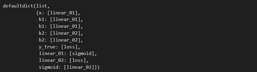
import networkx as nx
%matplotlib inline

graph = nx.DiGraph(computer_graph)
layout = nx.layout.spring_layout(graph)

nx.draw(graph, layout, with_labels=True)
给出图的一个拓扑排序
order = [node_x, node_k1, node_b1, node_linear01, node_sigmoid, node_k2, node_b2, node_linear02, node_y_true, node_loss]
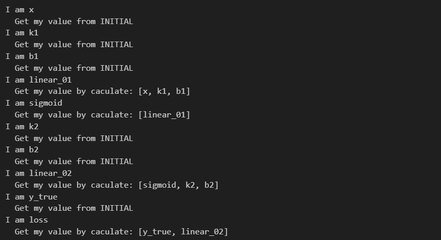
前向传播,用于计算loss
for node in order:
    print('I am {}'.format(node))
    node.forward()
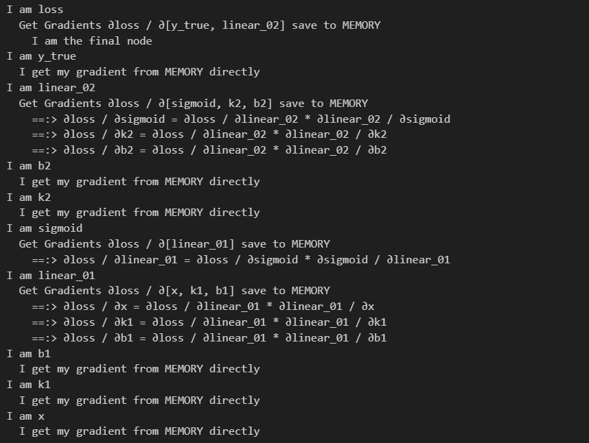
后向传播,用于计算偏导
for node in order[::-1]:
    print('I am {}'.format(node))
    node.backward()
我们要计算的其实就是 ∂loss / ∂[Placeholder],计算方式是链式求导,具体过程在下面的打印内容已经说的很清楚了
这里要体会两点
- 自动求导的代码框架,也就是Pytorch和TensorFlow等深度学习框架到底为我们做了什么
- 后向传播是如何将这么复杂的求导给简化的,每一步计算是如何参与下一步计算的
上面就是前向传播和后向传播的逻辑,接下来要落实的就是:
- forward calculate: function
- backward: gradient
- get order
Build a Neural Network
- Topological Sort
- Optimizer
- Batch Training
- Predict using neural network
- Multi-Dimension Neural Network
- How to distribute package
- How to compute image and text
拓扑排序算法 Get Order
while G:
- 找出所有出度不为0的节点
- 找出所有入度不为0的节点
- 选择一个入度为0的节点
- 删掉该节点
我们看一下怎么找只有出边没有入边的节点
from functools import reduce

set(computer_graph.keys())
### Output:
### {b1, b2, k1, k2, linear_01, linear_02, sigmoid, x, y_true}

computer_graph.values()
### Output:
### dict_values([[linear_01], [linear_01], [linear_01], [sigmoid], [linear_02], [linear_02], [linear_02], [loss], [loss]])

set(reduce(lambda x, y: x+y, computer_graph.values()))
### Output:
### {linear_01, linear_02, loss, sigmoid}

set(computer_graph.keys()) - set(reduce(lambda x, y: x+y, computer_graph.values()))
### Output:
### {b1, b2, k1, k2, x, y_true}
显然只要把{出度不为0的节点} - {入度不为0的节点}即可,所以
from functools import reduce
from operator import add

def topologic(graph):
    order = []
    while graph:
        all_nodes_have_outputs = set(graph.keys())
        all_nodes_have_inputs = set(reduce(add, graph.values()))

        nodes_only_have_outputs_no_input = all_nodes_have_outputs - all_nodes_have_inputs

        if nodes_only_have_outputs_no_input:
            n = random.choice(list(nodes_only_have_outputs_no_input))
            print('Get node: {}'.format(n))
            order.append(n)
            if len(graph) == 1:
                order += graph[n]  # order.append(graph[n][0])

            graph.pop(n)
            for _, links in graph.items():
                if n in links: links.remove(n)
        else:
            raise TypeError('This graph cannot get topologic order, which has a circle')
    return order
order = topologic(computer_graph)
order
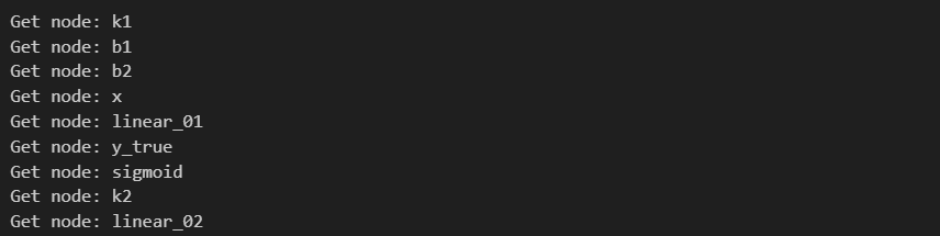

我们之所以要让计算机自己完成拓扑排序,是因为现实生活中我们构建的神经网络肯定不会像上面那么简单
from collections import defaultdict

nodes = ['node_{}'.format(i) for i in range(40)]
random.shuffle(nodes)

random_graph = defaultdict(list)

for i, n in enumerate(nodes):
    if i < len(nodes) - 1:
        random_graph[n] += random.sample(nodes[i+1:], k=random.randint(1, min(len(nodes) - (i+1), 3)))

graph = nx.DiGraph(random_graph)
laylout = nx.layout.spring_layout(graph)

nx.draw(graph, with_labels=True, node_size=25)
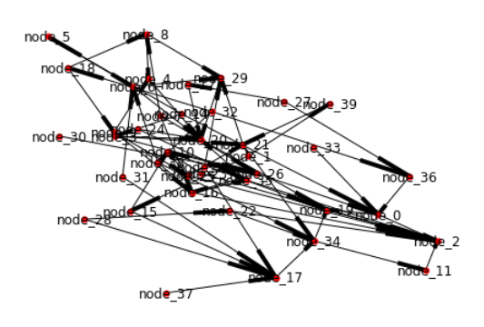
上面还只是40个节点的随机连线,要知道著名的神经网络RESNET光层数就有1000多层。
前向传播 & 后向传播 Feedforward & Feedbackward
前向传播 Feedforward
先来讲前向传播,为了清晰我们把backward函数都先pass掉。
前向传播具体增加的代码后面都有注释,就是读取输入然后根据函数 (线性/激活/Loss) 进行相应的计算
class Node:
    def __init__(self, name, inputs=[]):
        self.name = name
        self.inputs = inputs
        self.outputs = []
        self.value = None  # 用于前向传播计算值
        self.gradients = dict()  # loss对于每一个key的偏导

        for node in self.inputs:
            node.outputs.append(self)

    def forward(self):
        print('Get self value'.format(self))

    def backward(self):
        pass

    def __repr__(self):
        return self.name


class Placeholder(Node):
    def __init__(self, name):
        Node.__init__(self, name=name)

    def forward(self):
        print('  Get my value from INITIAL')

    def backward(self):
        print('  I get my gradient from MEMORY directly')

    def __repr__(self):
        return 'Placeholder: {}'.format(self.name)


class Linear(Node):  # Operator
    def __init__(self, name, inputs=[]):
        Node.__init__(self, name=name, inputs=inputs)

    def forward(self):
        print('  Get my value by caculate: {}'.format(self.inputs))
        x, k, b = self.inputs[0], self.inputs[1], self.inputs[2]
        self.value = k.value * x.value + b.value  # 线性函数的输出值

    def backward(self):
        pass

    def __repr__(self):
        return 'Linear: {}'.format(self.name)


class Sigmoid(Node):  # Operator
    def __init__(self, name, inputs=[]):
        Node.__init__(self, name=name, inputs=inputs)

    def _sigmoid(self, x):  # 定义激活函数_sigmoid
        return 1 / (1 + np.exp(-x))

    def forward(self):
        print('  Get my value by caculate: {}'.format(self.inputs))
        x = self.inputs[0]
        self.value = self._sigmoid(x.value)  # 激活函数的输出值

    def backward(self):
        pass

    def __repr__(self):
        return 'Sigmoid: {}'.format(self.name)


class Loss(Node):  # Operator
    def __init__(self, name, inputs=[]):
        Node.__init__(self, name=name, inputs=inputs)

    def forward(self):
        print('  Get my value by caculate: {}'.format(self.inputs))
        y = self.inputs[0]
        yhat = self.inputs[1]
        self.value = np.mean((y.value - yhat.value)**2)  # 求Loss

    def backward(self):
        pass

    def __repr__(self):
        return 'Loss: {}'.format(self.name)
初始化,跟之前一样,用 Linear/Sigmoid/Loss 替换Operator
node_x = Placeholder('x')
node_k1 = Placeholder('k1')
node_b1 = Placeholder('b1')
node_linear01 = Linear('linear_01', inputs=[node_x, node_k1, node_b1])
node_sigmoid = Sigmoid('sigmoid', inputs=[node_linear01])
node_k2 = Placeholder('k2')
node_b2 = Placeholder('b2')
node_linear02 = Linear('linear_02', inputs=[node_sigmoid, node_k2, node_b2])
node_y_true = Placeholder('y_true')
node_loss = Loss('loss', inputs=[node_y_true, node_linear02])
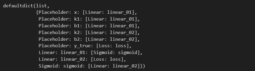
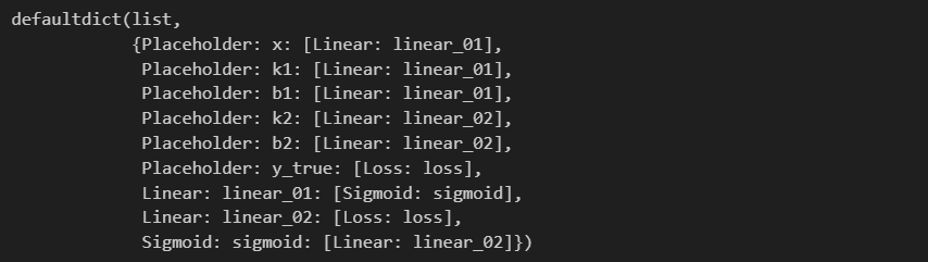
根据初始化信息生成图graph,遇到placeholder就用我们的feed_dict给它赋值
def convert_all_to_graph(feed):  # 用于自动生成我们之前的computer_graph
    computing_graph = defaultdict(list)

    need_expand = list(feed.keys())

    while need_expand:
        n = need_expand.pop(0)

        if n in computing_graph: continue

        if isinstance(n, Placeholder):  # 如果是placeholder就给它赋初始值
            n.value = feed[n]

        for m in n.outputs:
            computing_graph[n].append(m)
            need_expand.append(m)  # 别忘了将outputs中的内容加入搜索列表,这样才能找到所有连接关系

    return computing_graph
这里我们的feed_dict先用随机数
feed_dict = {
    node_x: 3,
    node_k1: random.random(),
    node_b1: random.random(),
    node_k2: random.random(),
    node_b2: random.random(),
    node_y_true: 0.38
}
computing_graph = convert_all_to_graph(feed_dict)
computing_graph
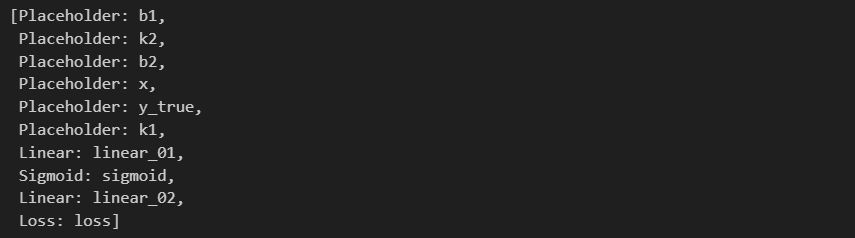
然后就是我们之前说过的拓扑排序算法,根据graph找到拓扑序列(代码完全一致,这里不再重复)
def topologic(graph):
    order = []
    while graph:
        ...
    return order
order = topologic(computing_graph)
order
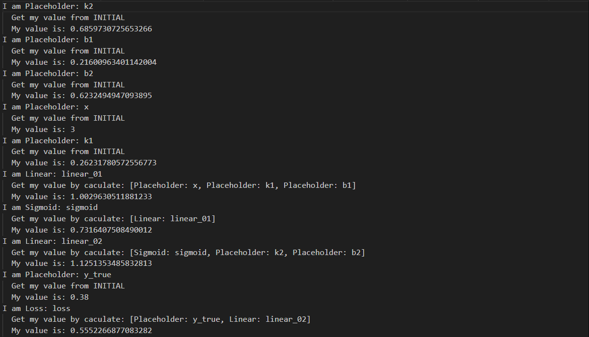
最后,前向传播,打印一下各placeholder和operator的值看看
for node in order:
    print('I am {}'.format(node))
    node.forward()
    print('  My value is: {}'.format(node.value))
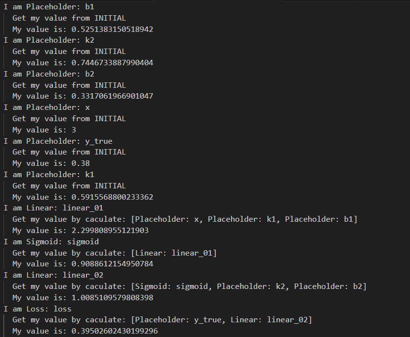
我们通过前向传播计算得到了loss值,每个函数和参数都被赋上了值,可喜可贺。
后向传播 Feedbackward
后向传播比前向传播要复杂,我们拆开来讲。
Loss
首先对于Loss对象,还记得我们在前后向传播原理部分打印过后向传播的输出吗?第一步是要计算 ∂loss / ∂[y_true, linear_02],具体实现就是对y和yhat求导 (根据我们的loss函数求导就行) 然后保存到 gradients 里去 (gradients里存的是loss对各节点的偏导)
loss=1n∑i=1n(yi−yhati)2 loss=\frac{1}{n}\sum_{i=1}^n(y_i-yhat_i)^2 loss=n1i=1∑n(yi−yhati)2
class Loss(Node):  # Operator
    # ...
    def backward(self):
        print('  Get Gradients ∂loss / ∂{} save to self.gradients'.format(self.inputs))
        # 对应之前的输出  Get Gradients ∂loss / ∂[y_true, linear_02] save to MEMORY
        y = self.inputs[0]
        yhat = self.inputs[1]
        self.gradients[y] = 2 * np.mean(y.value - yhat.value)
        self.gradients[yhat] = -2 * np.mean(y.value - yhat.value)
Linear
接下来我们处理Linear对象,这步的代码实现个人觉得比较难懂,一定要仔细理解!
在Linear中,我们有3个参数k、x、b,因此分别要求 ∂loss / ∂[k, x, b]。以 ∂loss/∂k 为例,链式求导过程为 ∂loss/∂linear * ∂linear/∂k。
因为我们现在自己就是Linear对象中的方法,所以可以写成 ∂loss/∂self * ∂self/∂k,其中 ∂loss/∂self 是 gradients[self],而∂self/∂k 就是 x。
那么我们现在唯一的问题就是 gradients[self] 如何求解,也就是 ∂loss/∂linear 是什么?
哈哈,其实我们在之前Loss对象的处理过程中已经计算出来了,这就是反向传播/后向传播的魅力,它在逻辑上几乎就是前向传播的逆过程。
因此,gradients[self] = self.outputs[0].gradients[self],这段代码的意思就是找到Linear的输出 (也就是Loss) 关于Linear的偏导,赋值给 gradients[self] 作为∂loss/∂linear。
综上,gradients[k] = self.outputs[0].gradients[self] * x.value。同理 x、b。
class Linear(Node):  # Operator
    # ...
    def backward(self):
        print('  Get Gradients ∂loss / ∂{} save to MEMORY'.format(self.inputs))
        x, k, b = self.inputs[0], self.inputs[1], self.inputs[2]

        self.gradients[k] = self.outputs[0].gradients[self] * x.value
        self.gradients[x] = self.outputs[0].gradients[self] * k.value
        self.gradients[b] = self.outputs[0].gradients[self] * 1
Sigmoid
同样的,来看一下Sigmoid,要求 ∂loss/∂xx,即求 ∂loss/∂linear * ∂linear/∂x * ∂x/∂xx,其中 ∂loss/∂linear * ∂linear/∂x = ∂loss/∂x 已在上一步求得,因此
class Sigmoid(Node):  # Operator
    def _sigmoid(self, x):  # 定义激活函数_sigmoid
        return 1 / (1 + np.exp(-x))
	# ...
    def backward(self):
        print('  Get Gradients ∂loss / ∂{} save to MEMORY'.format(self.inputs))
        xx = self.inputs[0]

        self.gradients[xx] = self.outputs[0].gradients[self] * self._sigmoid(xx.value) * (1 - self._sigmoid(xx.value))
数学基础:Sigmoid求导
S′(x)=−1(1+e−x)2×(1+e−x)′=−1(1+e−x)2×(−e−x)=1(1+e−x)×1+e−x−1(1+e−x)=S(x)(1−S(x)) \begin{align} S'(x) &= -\frac{1}{(1+e^{-x})^2}\times(1+e^{-x})' \\&= -\frac{1}{(1+e^{-x})^2}\times(-e^{-x}) \\&= \frac{1}{(1+e^{-x})}\times \frac{1+e^{-x}-1}{(1+e^{-x})}\\&= S(x)(1-S(x)) \end{align} S′(x)=−(1+e−x)21×(1+e−x)′=−(1+e−x)21×(−e−x)=(1+e−x)1×(1+e−x)1+e−x−1=S(x)(1−S(x))
Placeholder
最后是Placeholder
class Placeholder(Node):
    # ...
    def backward(self):
        print('  I get my gradient from MEMORY directly')
        self.gradients[self] = self.outputs[0].gradients[self]
拆开来搞清楚了,接下来就是合起来。
下面是完整前后向传播代码
class Node:
    def __init__(self, name, inputs=[]):
        self.name = name
        self.inputs = inputs
        self.outputs = []
        self.value = None  # 用于前向传播计算值
        self.gradients = dict()  # loss对于每一个key的偏导

        for node in self.inputs:
            node.outputs.append(self)

    def forward(self):
        print('Get self value'.format(self))

    def backward(self):
        pass

    def __repr__(self):
        return self.name


class Placeholder(Node):
    def __init__(self, name):
        Node.__init__(self, name=name)

    def forward(self):
        print('  Get my value from INITIAL')

    def backward(self):
        print('  I get my gradient from MEMORY directly')
        self.gradients[self] = self.outputs[0].gradients[self]

    def __repr__(self):
        return 'Placeholder: {}'.format(self.name)


class Linear(Node):  # Operator
    def __init__(self, name, inputs=[]):
        Node.__init__(self, name=name, inputs=inputs)

    def forward(self):
        print('  Get my value by caculate: {}'.format(self.inputs))
        x, k, b = self.inputs[0], self.inputs[1], self.inputs[2]
        self.value = k.value * x.value + b.value  # 线性函数的输出值

    def backward(self):
        print('  Get Gradients ∂loss / ∂{} save to MEMORY'.format(self.inputs))
        x, k, b = self.inputs[0], self.inputs[1], self.inputs[2]

        self.gradients[k] = self.outputs[0].gradients[self] * x.value
        self.gradients[x] = self.outputs[0].gradients[self] * k.value
        self.gradients[b] = self.outputs[0].gradients[self] * 1


    def __repr__(self):
        return 'Linear: {}'.format(self.name)


class Sigmoid(Node):  # Operator
    def __init__(self, name, inputs=[]):
        Node.__init__(self, name=name, inputs=inputs)

    def _sigmoid(self, x):  # 定义激活函数_sigmoid
        return 1 / (1 + np.exp(-x))

    def forward(self):
        print('  Get my value by caculate: {}'.format(self.inputs))
        x = self.inputs[0]
        self.value = self._sigmoid(x.value)  # 激活函数的输出值

    def backward(self):
        print('  Get Gradients ∂loss / ∂{} save to MEMORY'.format(self.inputs))
        xx = self.inputs[0]

        self.gradients[xx] = self.outputs[0].gradients[self] * self._sigmoid(xx.value) * (1 - self._sigmoid(xx.value))

    def __repr__(self):
        return 'Sigmoid: {}'.format(self.name)


class Loss(Node):  # Operator
    def __init__(self, name, inputs=[]):
        Node.__init__(self, name=name, inputs=inputs)

    def forward(self):
        print('  Get my value by caculate: {}'.format(self.inputs))
        y = self.inputs[0]
        yhat = self.inputs[1]
        self.value = np.mean((y.value - yhat.value)**2)  # 求Loss

    def backward(self):
        print('  Get Gradients ∂loss / ∂{} save to self.gradients'.format(self.inputs))
        # 对应之前的输出  Get Gradients ∂loss / ∂[y_true, linear_02] save to MEMORY
        y = self.inputs[0]
        yhat = self.inputs[1]
        self.gradients[y] = 2 * np.mean(y.value - yhat.value)
        self.gradients[yhat] = -2 * np.mean(y.value - yhat.value)

    def __repr__(self):
        return 'Loss: {}'.format(self.name)
node_x = Placeholder('x')
node_k1 = Placeholder('k1')
node_b1 = Placeholder('b1')
node_linear01 = Linear('linear_01', inputs=[node_x, node_k1, node_b1])
node_sigmoid = Sigmoid('sigmoid', inputs=[node_linear01])
node_k2 = Placeholder('k2')
node_b2 = Placeholder('b2')
node_linear02 = Linear('linear_02', inputs=[node_sigmoid, node_k2, node_b2])
node_y_true = Placeholder('y_true')
node_loss = Loss('loss', inputs=[node_y_true, node_linear02])
def convert_all_to_graph(feed):  # 用于自动生成我们之前的computer_graph
    computing_graph = defaultdict(list)

    need_expand = list(feed.keys())

    while need_expand:
        n = need_expand.pop(0)

        if n in computing_graph: continue

        if isinstance(n, Placeholder):  # 如果是placeholder就给它赋初始值
            n.value = feed[n]

        for m in n.outputs:
            computing_graph[n].append(m)
            need_expand.append(m)  # 别忘了将outputs中的内容加入搜索列表,这样才能找到所有连接关系

    return computing_graph
feed_dict = {
    node_x: 3,
    node_k1: random.random(),
    node_b1: random.random(),
    node_k2: random.random(),
    node_b2: random.random(),
    node_y_true: 0.38
}
computing_graph = convert_all_to_graph(feed_dict)
computing_graph
from operator import add

def topologic(graph):
    order = []
    while graph:
        all_nodes_have_outputs = set(graph.keys())
        all_nodes_have_inputs = set(reduce(add, graph.values()))

        nodes_only_have_outputs_no_input = all_nodes_have_outputs - all_nodes_have_inputs

        if nodes_only_have_outputs_no_input:
            n = random.choice(list(nodes_only_have_outputs_no_input))
            # print('Get node: {}'.format(n))
            order.append(n)
            if len(graph) == 1:
                order += graph[n]  # order.append(graph[n][0])

            graph.pop(n)
            for _, links in graph.items():
                if n in links: links.remove(n)
        else:
            raise TypeError('This graph cannot get topologic order, which has a circle')
    return order
order = topologic(computing_graph)

for node in order:
    print('I am {}'.format(node))
    node.forward()
    print('  My value is: {}'.format(node.value))

for node in order[::-1]:
    print('I am {}'.format(node))
    node.backward()
    print('  Get Gradients: {}'.format(node.gradients))
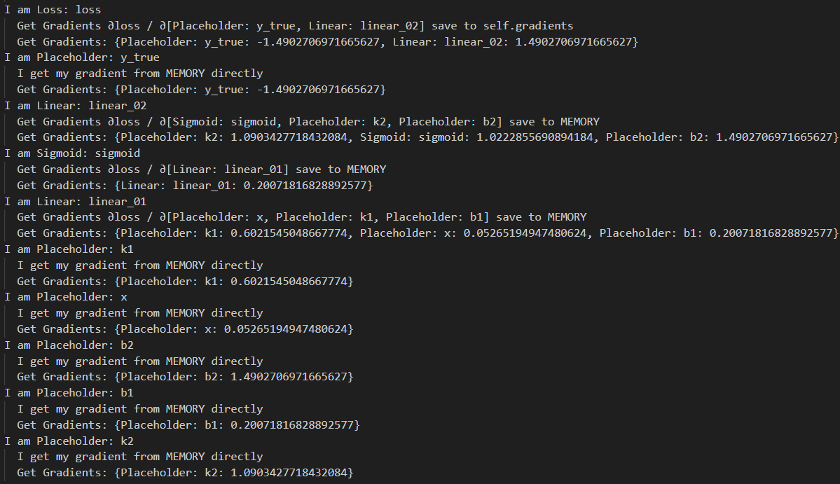
最终输出如上,我们通过后向传播得到了loss对所有参数的导数 (合理的是计算顺序符合y_true/linear_02 -> sigmoid/k2/b2 -> linear_01 -> x/k1/b1),有了这些导数,我们终于可以愉快地梯度下降啦~
优化 Optimize
有了这些导数,我们要用它们来对参数进行更新。
仔细想想,我们要更新的参数其实就是k和·b,x和y_true是不更新的,所以我们有必要在Placeholder类的定义中将两者区分开来。
class Node:
    def __init__(self, name, inputs=[], is_trainable=False):
        self.name = name
        self.inputs = inputs
        self.outputs = []
        self.value = None  # 用于前向传播计算值
        self.gradients = dict()  # loss对于每一个key的偏导
        self.is_trainable = is_trainable

        for node in self.inputs:
            node.outputs.append(self)

    def forward(self):
        # print('Get self value'.format(self))
        pass

    def backward(self):
        pass

    def __repr__(self):
        return self.name


class Placeholder(Node):
    def __init__(self, name, is_trainable=True):
        Node.__init__(self, name=name, is_trainable=is_trainable)

    def forward(self):
        # print('  Get my value from INITIAL')
        pass

    def backward(self):
        # print('  I get my gradient from MEMORY directly')
        pass
        self.gradients[self] = self.outputs[0].gradients[self]

    def __repr__(self):
        return 'Placeholder: {}'.format(self.name)
加上is_trainable属性重新定义一下各Placeholder
node_x = Placeholder('x', is_trainable=False)
node_k1 = Placeholder('k1', is_trainable=True)
node_b1 = Placeholder('b1', is_trainable=True)
node_linear01 = Linear('linear_01', inputs=[node_x, node_k1, node_b1])
node_sigmoid = Sigmoid('sigmoid', inputs=[node_linear01])
node_k2 = Placeholder('k2', is_trainable=True)
node_b2 = Placeholder('b2', is_trainable=True)
node_linear02 = Linear('linear_02', inputs=[node_sigmoid, node_k2, node_b2])
node_y_true = Placeholder('y_true', is_trainable=False)
node_loss = Loss('loss', inputs=[node_y_true, node_linear02])
feed_dict = {
    node_x: 3,
    node_k1: random.random(),
    node_b1: random.random(),
    node_k2: random.random(),
    node_b2: random.random(),
    node_y_true: 0.38
}
computing_graph = convert_all_to_graph(feed_dict)
我们将前向传播、后向传播和优化分别封装成函数,只打印Loss函数的值便于观察变化
order = topologic(computing_graph)

def feedforward(order_nodes):
    for node in order_nodes:
        # print('I am {}'.format(node))
        node.forward()
        if isinstance(node, Loss):
            print('  My value is: {}'.format(node.value))

def feedbackward(order_nodes):
    for node in order_nodes[::-1]:
        # print('I am {}'.format(node))
        node.backward()
        # print('  Get Gradients: {}'.format(node.gradients))

def optimize(order_nodes, learning_rate=1e-3):
    for node in order_nodes:
        if node.is_trainable:
            node.value = node.value + (-1) * node.gradients[node] * learning_rate
            print('Update node: {} value = {}.value + (-1) * ∂loss / ∂{}'.format(node, node, node))
先迭代10次
for i in range(10):
    print('Epoch: {}'.format(i))
    feedforward(order)
    feedbackward(order)
    optimize(order)
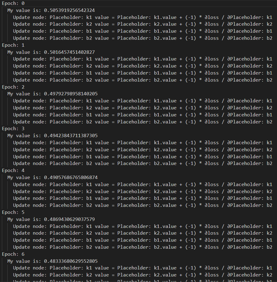
结果就是不断更新参数k和b,使得loss值越来越小。学习率1e-3迭代10次,loss值从0.505下降到了0.472。
删去不必要的输出,修改学习率为1e-1迭代50次
for i in range(50):
    print('Epoch: {}'.format(i))
    feedforward(order)
    feedbackward(order)
    optimize(order, learning_rate=1e-1)
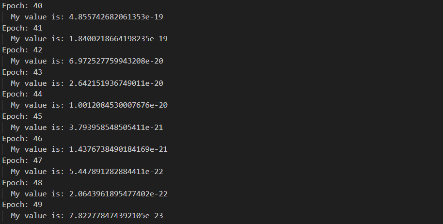
loss值最终下降到了7.822e-23。
打印一下yhat (也就是Linear_02的输出值) 看看
order[-2].value

非常接近我们设置的y_true,也就是0.38。
至此,我们手工实现了一个一维的深度学习网络。
波士顿房价
下面我们用我们手搓的深度学习网络对波士顿房价进行预测。
from sklearn.datasets import load_boston
data = load_boston()

X_rm, y_ = data['data'][:,5], data['target']  # X_rm为数据第6列

node_x = Placeholder('x', is_trainable=False)
node_k1 = Placeholder('k1', is_trainable=True)
node_b1 = Placeholder('b1', is_trainable=True)
node_linear01 = Linear('linear_01', inputs=[node_x, node_k1, node_b1])
node_sigmoid = Sigmoid('sigmoid', inputs=[node_linear01])
node_k2 = Placeholder('k2', is_trainable=True)
node_b2 = Placeholder('b2', is_trainable=True)
node_linear02 = Linear('linear_02', inputs=[node_sigmoid, node_k2, node_b2])
node_y_true = Placeholder('y_true', is_trainable=False)
node_loss = Loss('loss', inputs=[node_y_true, node_linear02])

feed_dict = {
    node_x: X_rm,
    node_k1: random.random(),
    node_b1: random.random(),
    node_k2: random.random(),
    node_b2: random.random(),
    node_y_true: y_
}

computing_graph = convert_all_to_graph(feed_dict)

order = topologic(computing_graph)
from tqdm import tqdm_notebook # 加个进度条 不然等待运行的过程很折磨
def run_one_epoch(order_nodes):
    feedforward(order_nodes)
    feedbackward(order_nodes)
epoch = 1000
batch_num = len(X_rm)
losses = []

for e in tqdm_notebook(range(epoch)):
    loss = 0
    for b in range(batch_num):  # 分批载入数据
        index = np.random.choice(range(len(X_rm)))
        node_x.value = X_rm[index]
        node_y_true.value = y_[index]

        run_one_epoch(order)
        optimize(order, learning_rate=1e-3)

        loss += node_loss.value

    losses.append(loss / batch_num)
plt.plot(losses)
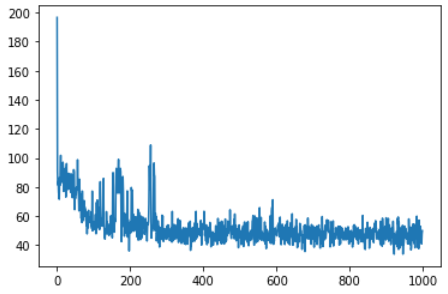
可以看到实现了梯度下降,最后仍有波动的原因显然是因为房价是由多个维度的因素决定的 (数据集给了13个维度),而我们这里只用了1个维度,所以梯度下降顶天也只能优化到这个程度。
我们可以预测一下房价看看
def predict(x):
    node_x.value = x
    feedforward(order)
    return node_linear02.value
predict(7)
### Output:
### 32.392347322443726
plt.scatter(X_rm, y_)
plt.scatter(X_rm, [predict(x_) for x_ in X_rm])
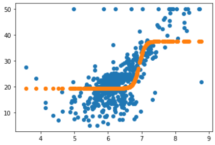
可以看到这就是我们拟合出来的曲线,相比于最开始线性函数的预测效果会好很多。
多维函数拟合
多维拟合
之前也提到了,我们现在只用了一维的数据进行拟合,效果比线性函数好但仍旧不是很理想。
这里将代码改成多维,思路和一维是一样的
import numpy as np
import random

class Node:
    def __init__(self, inputs=[]):
        self.inputs = inputs
        self.outputs = []

        for n in self.inputs:
            n.outputs.append(self)
            # set 'self' node as inbound_nodes's outbound_nodes

        self.value = None

        self.gradients = {}
        # keys are the inputs to this node, and their
        # values are the partials of this node with
        # respect to that input.
        # \partial{node}{input_i}


    def forward(self):
        '''
        Forward propagation.
        Compute the output value vased on 'inbound_nodes' and store the
        result in self.value
        '''
        raise NotImplemented


    def backward(self):

        raise NotImplemented

class Placeholder(Node):
    def __init__(self):
        '''
        An Input node has no inbound nodes.
        So no need to pass anything to the Node instantiator.
        '''
        Node.__init__(self)

    def forward(self, value=None):
        '''
        Only input node is the node where the value may be passed
        as an argument to forward().
        All other node implementations should get the value of the
        previous node from self.inbound_nodes

        Example:
        val0: self.inbound_nodes[0].value
        '''
        if value is not None:
            self.value = value
            ## It's is input node, when need to forward, this node initiate self's value.

        # Input subclass just holds a value, such as a data feature or a model parameter(weight/bias)

    def backward(self):
        self.gradients = {self:0}
        for n in self.outputs:
            grad_cost = n.gradients[self]
            self.gradients[self] = grad_cost * 1


class Add(Node):
    def __init__(self, *nodes):
        Node.__init__(self, nodes)

    def forward(self):
        self.value = sum(map(lambda n: n.value, self.inputs))
        ## when execute forward, this node caculate value as defined.


class Linear(Node):
    def __init__(self, nodes, weights, bias):
        Node.__init__(self, [nodes, weights, bias])

    def forward(self):
        inputs = self.inputs[0].value
        weights = self.inputs[1].value
        bias = self.inputs[2].value

        self.value = np.dot(inputs, weights) + bias

    def backward(self):
        # initial a partial for each of the inbound_nodes.
        self.gradients = {n: np.zeros_like(n.value) for n in self.inputs}

        for n in self.outputs:
            # Get the partial of the cost w.r.t this node.
            grad_cost = n.gradients[self]
            # 与一维的区别在于这里使用点乘dot
            self.gradients[self.inputs[0]] = np.dot(grad_cost, self.inputs[1].value.T)
            self.gradients[self.inputs[1]] = np.dot(self.inputs[0].value.T, grad_cost)
            self.gradients[self.inputs[2]] = np.sum(grad_cost, axis=0, keepdims=False)


class Sigmoid(Node):
    def __init__(self, node):
        Node.__init__(self, [node])

    def _sigmoid(self, x):
        return 1./(1 + np.exp(-1 * x))

    def forward(self):
        self.x = self.inputs[0].value
        self.value = self._sigmoid(self.x)

    def backward(self):
        self.partial = self._sigmoid(self.x) * (1 - self._sigmoid(self.x))

        self.gradients = {n: np.zeros_like(n.value) for n in self.inputs}

        for n in self.outputs:
            grad_cost = n.gradients[self]  # Get the partial of the cost with respect to this node.

            self.gradients[self.inputs[0]] = grad_cost * self.partial
            # use * to keep all the dimension same!.


class MSE(Node):  # Loss
    def __init__(self, y, yhat):
        Node.__init__(self, [y, yhat])

    def forward(self):
        y = self.inputs[0].value.reshape(-1, 1)
        yhat = self.inputs[1].value.reshape(-1, 1)
        assert(y.shape == yhat.shape)

        self.m = self.inputs[0].value.shape[0]
        self.diff = y - yhat

        self.value = np.mean(self.diff**2)

    def backward(self):
        self.gradients[self.inputs[0]] = (2 / self.m) * self.diff
        self.gradients[self.inputs[1]] = (-2 / self.m) * self.diff


def forward_and_backward(graph):
    # execute all the forward method of sorted_nodes.

    ## In practice, it's common to feed in mutiple data example in each forward pass rather than just 1. Because the examples can be processed in parallel. The number of examples is called batch size.
    for n in graph:
        n.forward()
        ## each node execute forward, get self.value based on the topological sort result.

    for n in  graph[::-1]:
        n.backward()


def toplogic(graph):
    sorted_node = []

    while len(graph) > 0:
        all_inputs = []
        all_outputs = []

        for n in graph:
            all_inputs += graph[n]
            all_outputs.append(n)

        all_inputs = set(all_inputs)
        all_outputs = set(all_outputs)

        need_remove = all_outputs - all_inputs  # which in all_inputs but not in all_outputs

        if len(need_remove) > 0:
            node = random.choice(list(need_remove))
            need_to_visited = [node]

            if len(graph) == 1: need_to_visited += graph[node]

            graph.pop(node)
            sorted_node += need_to_visited

            for _, links in graph.items():
                if node in links: links.remove(node)
        else: # have cycle
            break

    return sorted_node


from collections import defaultdict

def convert_feed_dict_to_graph(feed_dict):
    computing_graph = defaultdict(list)
    nodes = [n for n in feed_dict]

    while nodes:
        n = nodes.pop(0)

        if isinstance(n, Placeholder):
            n.value = feed_dict[n]

        if n in computing_graph: continue

        for m in n.outputs:
            computing_graph[n].append(m)
            nodes.append(m)

    return computing_graph

def topological_sort_feed_dict(feed_dict):
    graph = convert_feed_dict_to_graph(feed_dict)

    return toplogic(graph)


def optimize(trainables, learning_rate=1e-2):
    # there are so many other update / optimization methods
    # such as Adam, Mom, ...
    for t in trainables:
        t.value += -1 * learning_rate * t.gradients[t]
import numpy as np
from sklearn.datasets import load_boston
from sklearn.utils import shuffle, resample
from tqdm import tqdm_notebook
#from miniflow import *

# Load data
data = load_boston()
X_ = data['data']
y_ = data['target']

# Normalize data
X_ = (X_ - np.mean(X_, axis=0)) / np.std(X_, axis=0)

n_features = X_.shape[1]
n_hidden = 10
W1_ = np.random.randn(n_features, n_hidden)
b1_ = np.zeros(n_hidden)
W2_ = np.random.randn(n_hidden, 1)
b2_ = np.zeros(1)

# Neural network
X, y = Placeholder(), Placeholder()
W1, b1 = Placeholder(), Placeholder()
W2, b2 = Placeholder(), Placeholder()

l1 = Linear(X, W1, b1)
s1 = Sigmoid(l1)
l2 = Linear(s1, W2, b2)
cost = MSE(y, l2)

feed_dict = {
    X: X_,
    y: y_,
    W1: W1_,
    b1: b1_,
    W2: W2_,
    b2: b2_
}

epochs = 5000
# Total number of examples
m = X_.shape[0]
batch_size = 16
steps_per_epoch = m // batch_size

graph = topological_sort_feed_dict(feed_dict)
trainables = [W1, b1, W2, b2]

print("Total number of examples = {}".format(m))
### Output:
### Total number of examples = 506
losses = []

for i in tqdm_notebook(range(epochs)):
    loss = 0
    for j in range(steps_per_epoch):
        # Step 1
        # Randomly sample a batch of examples
        X_batch, y_batch = resample(X_, y_, n_samples=batch_size)
        # Reset value of X and y Inputs
        X.value = X_batch
        y.value = y_batch

        # Step 2
        forward_and_backward(graph) # set output node not important.

        # Step 3
        rate = 1e-2
        optimize(trainables, rate)

        loss += graph[-1].value

    if i % 100 == 0:
        print("Epoch: {}, Loss: {:.3f}".format(i+1, loss/steps_per_epoch))
        losses.append(loss/steps_per_epoch)
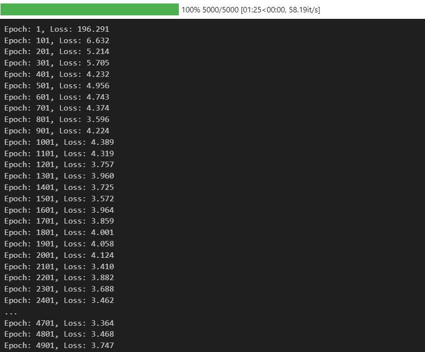
plt.plot(losses)
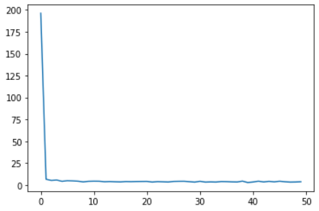
明显下降效果相较之前有所提升。
二维效果
由于13维对我们来说不能直观看到,我们选其中的两个维度来看看。
import pandas as pd

dataframe = pd.DataFrame(data['data'])
dataframe.columns = data['feature_names']

training_data = dataframe[['RM', 'LSTAT']]
import numpy as np
from sklearn.datasets import load_boston
from sklearn.utils import shuffle, resample
#from miniflow import *

# Load data
data = load_boston()
X_ = training_data
y_ = data['target']

# Normalize data
X_ = (X_ - np.mean(X_, axis=0)) / np.std(X_, axis=0)

n_features = X_.shape[1]
n_hidden = 10
W1_ = np.random.randn(n_features, n_hidden)
b1_ = np.zeros(n_hidden)
W2_ = np.random.randn(n_hidden, 1)
b2_ = np.zeros(1)

# Neural network
X, y = Placeholder(), Placeholder()
W1, b1 = Placeholder(), Placeholder()
W2, b2 = Placeholder(), Placeholder()

l1 = Linear(X, W1, b1)
s1 = Sigmoid(l1)
l2 = Linear(s1, W2, b2)
cost = MSE(y, l2)

feed_dict = {
    X: X_,
    y: y_,
    W1: W1_,
    b1: b1_,
    W2: W2_,
    b2: b2_
}

epochs = 1000
# Total number of examples
m = X_.shape[0]
batch_size = 1
steps_per_epoch = m // batch_size

graph = topological_sort_feed_dict(feed_dict)
trainables = [W1, b1, W2, b2]
losses = []

for i in range(epochs):
    loss = 0
    for j in range(steps_per_epoch):
        # Step 1
        # Randomly sample a batch of examples
        X_batch, y_batch = resample(X_, y_, n_samples=batch_size)
        # Reset value of X and y Inputs
        X.value = X_batch
        y.value = y_batch

        # Step 2
        forward_and_backward(graph) # set output node not important.

        # Step 3
        rate = 1e-2
        optimize(trainables, rate)

        loss += graph[-1].value

    if i % 100 == 0:
        # print("Epoch: {}, Loss: {:.3f}".format(i+1, loss/steps_per_epoch))
        losses.append(loss/steps_per_epoch)
试试预测
X.value = np.array([[6, 8]])
forward_and_backward(graph)
graph[-2].value[0][0]
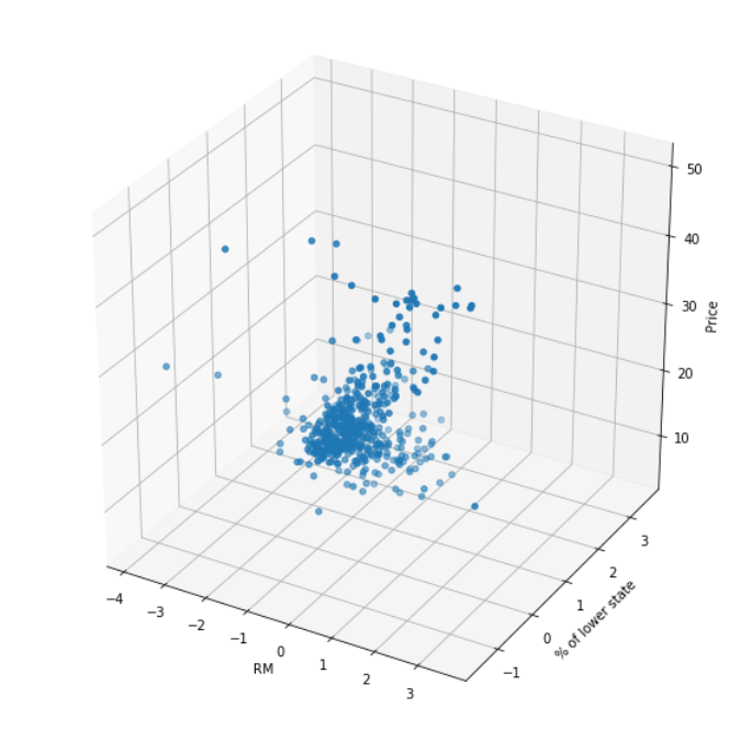
我们画一张3D图看看我们到底拟合出了什么东西
这里介绍一个python画图技巧
from mpl_toolkits.mplot3d import Axes3D
import matplotlib.pyplot as plt

fig = plt.figure()
ax = fig.gca(projection='3d')
from mpl_toolkits.mplot3d import Axes3D
import matplotlib.pyplot as plt
from matplotlib import cm
from matplotlib.ticker import LinearLocator, FormatStrFormatter
import numpy as np


fig = plt.figure(figsize=(10, 10))
ax = fig.add_subplot(111, projection='3d')

# Make data.
X = X_.values[:, 0]
Y = X_.values[:, 1]
Z = y_

# Plot the surface.
rm_and_lstp_price = ax.scatter(X, Y, Z)
ax.set_xlabel('RM')
ax.set_ylabel('% of lower state')
ax.set_zlabel('Price')
training_data.values
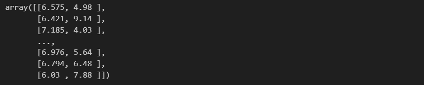
predicate_result = []
for rm, ls in training_data.values:
    X = np.array([[rm, ls]])
    forward_and_backward(graph)
    predicate_result.append(graph[-2].value[0][0])

predicate_result = np.array(predicate_result)
%matplotlib notebook
fig = plt.figure(figsize=(10, 10))
ax = fig.add_subplot(111, projection='3d')

# Make data.
X = X_.values[:, 0]
Y = X_.values[:, 1]
Z = predicate_result

# Plot the surface.
rm_and_lstp_price = ax.plot_trisurf(X, Y, Z, color='green')

ax.set_xlabel('RM')
ax.set_ylabel('% of lower state')
ax.set_zlabel('Predicated-Price')
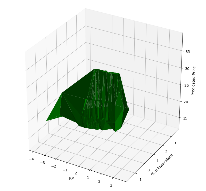
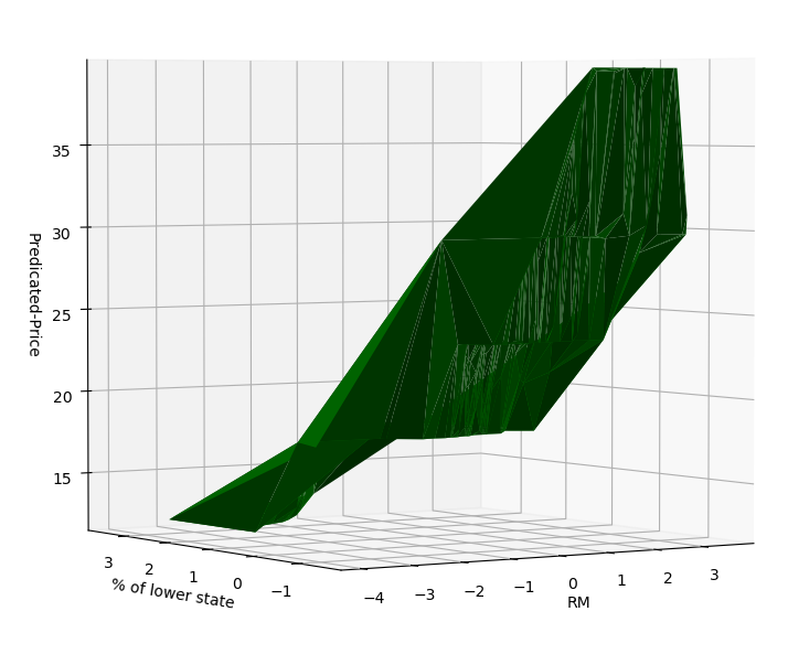
可以看出来,拟合得到的其实是一个三维空间中的曲面。
这个曲面在某种程度上也是可解释的
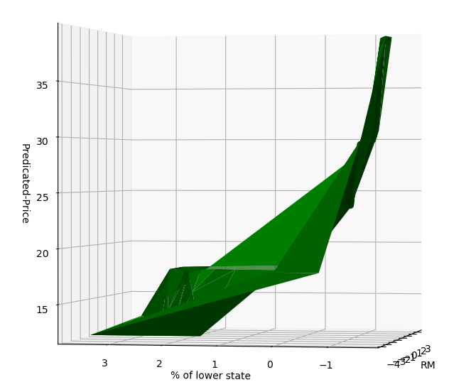
lower state占比越小,房价越高;
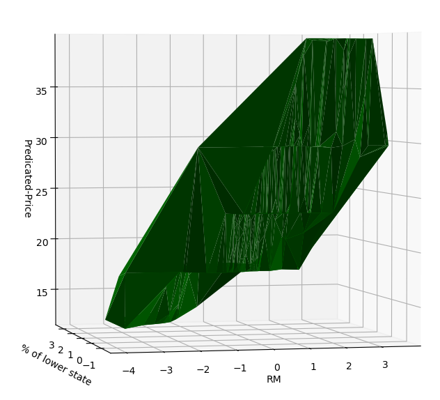
RM越大,房价越高。
而在多维拟合中最后得到的会是十三维的,这也就是为什么它的拟合效果会非常好。

技术共进,成长同行——讯飞AI开发者社区
更多推荐


 14
14 0
0- 0


 已为社区贡献1条内容

所有评论(0)