
机器学习库 | PyTorch:torch.nn
需安装torchinfo库# 定义网络nn.ReLU(),# 实例化网络# 显示模型摘要SimpleNetnn.init控制权重初始化策略# 定义网络# 自定义初始化init.xavier_normal_(self.fc.weight) # Xavier初始化init.constant_(self.fc.bias, 0.1) # 偏置初始化为0.1# 实例化网络# 查看参数print("权重初始化
torch.nn是PyTorch中构建神经网络的核心模块,提供了从基础层到复杂网络结构的完整工具链。
1、nn.Module
所有神经网络模块的基类,自定义网络需继承此类。
import torch
import torch.nn as nn

# 定义一个简单全连接网络
class SimpleNet(nn.Module):
    def __init__(self):
        super(SimpleNet, self).__init__() # super()函数需要知道当前类是谁,以便正确地找到父类的构造函数。父类的方法需要绑定到当前实例上,以便能够正确地调用。
        # 线性层:输入特征2,输出特征1
        self.fc1 = nn.Linear(2, 1)

    def forward(self, x):
        # 前向传播计算
        return self.fc1(x)

# 实例化网络
net = SimpleNet()
print(net)  # 打印网络结构


# SimpleNet(
  (fc1): Linear(in_features=2, out_features=1, bias=True)
)
2、核心层
2.1、线性层
nn.Linear(in_features, out_features):对输入数据进行线性变换 ![]()
# 创建线性层:输入维度3,输出维度2
linear = nn.Linear(3, 2)

# 输入数据(批量大小2,特征数3)
input_data = torch.tensor([[1.0, 2.0, 3.0], [4.0, 5.0, 6.0]])

# 前向传播
output = linear(input_data)
print("输出数据:\n", output)
print("输出形状:", output.shape)


输出数据:
 tensor([[ 2.7557, -0.8099],
         [ 7.3660, -3.1438]], grad_fn=<AddBackward0>)
输出形状: torch.Size([2, 2])
2.2、卷积层
| 卷积类型 | 空间维度 | 常见用途 | 输入张量形状示例 |
|---|---|---|---|
| 1D卷积 | 时间序列、文本等 | 序列数据处理 | (batch, in_channels, length) |
| 2D卷积 | 图像 | 图像识别、检测等 | (batch, in_channels, height, width) |
| 3D卷积 | 视频、医学图像等 | 视频分析、3D图像处理 | (batch, in_channels, depth, height, width) |
卷积核运算过程:
self.conv1d = nn.Conv1d(in_channels=3, out_channels=6, kernel_size=5)
- 输入数据:具有3个通道(比如时间序列数据的不同特征)。每个通道的数据长度为某个特定值(例如32)。
- 卷积核:总共有6个不同的卷积核(filters),每个卷积核负责生成输出中的一个通道。因此,输出将包含6个通道。
- 每个卷积核的结构:由于输入有3个通道,所以每个卷积核也需要对应这3个通道。每个卷积核在其对应的每个通道上有长度为5的权重(即每个通道上的局部感受野大小为5),这些权重会被用来与输入数据中相应通道的元素进行卷积操作。
具体到某一个卷积核的工作流程:
- 对于该卷积核,它会通过其三个通道的权重矩阵(每个大小为5)分别与输入数据的三个通道做卷积运算。
- 在每个位置上,卷积核的每个通道与输入数据对应通道的元素相乘后的结果会被加在一起,得到单个输出值。
- 重复这个过程,滑动卷积窗口遍历整个输入长度,产生输出通道的一个完整序列。
2.2.1、nn.Conv1d
nn.Conv1d是一维卷积层,常用于处理一维信号数据,如时间序列数据。参数
in_channels: 输入信号的通道数。out_channels: 输出信号的通道数。kernel_size: 卷积核的大小。stride: 卷积步长,默认为1。padding: 填充模式,默认为0。dilation: 空洞率,默认为1。groups: 分组数量,默认为1。bias: 是否使用偏置项,默认为True。
import torch
import torch.nn as nn

class Conv1DExample(nn.Module):
    def __init__(self):
        super(Conv1DExample, self).__init__()
        self.conv1d = nn.Conv1d(in_channels=3, out_channels=6, kernel_size=5)

    def forward(self, x):
        return self.conv1d(x)

# 创建一个输入张量,形状为 (batch_size, in_channels, length)
input_tensor = torch.randn(1, 3, 10)
model = Conv1DExample()
output = model(input_tensor)
print(output.shape) # 输出形状应为 (1, 6, 6)2.2.2、nn.Conv2d
nn.Conv2d是二维卷积层,常用于图像处理任务。参数
in_channels: 输入图像的通道数。out_channels: 输出图像的通道数。kernel_size: 卷积核的大小(可以是整数或元组)。stride: 卷积步长,默认为1。padding: 填充模式,默认为0。dilation: 空洞率,默认为1。groups: 分组数量,默认为1。bias: 是否使用偏置项,默认为True。
import torch
import torch.nn as nn

class Conv2DExample(nn.Module):
    def __init__(self):
        super(Conv2DExample, self).__init__()
        self.conv2d = nn.Conv2d(in_channels=3, out_channels=6, kernel_size=(5, 5))

    def forward(self, x):
        return self.conv2d(x)

# 创建一个输入张量,形状为 (batch_size, in_channels, height, width)
input_tensor = torch.randn(1, 3, 32, 32)
model = Conv2DExample()
output = model(input_tensor)
print(output.shape) # 输出形状应为 (1, 6, 28, 28)2.2.3、nn.Conv3d
nn.Conv3d是三维卷积层,常用于视频处理或其他三维数据处理任务。参数
in_channels: 输入体积的通道数。out_channels: 输出体积的通道数。kernel_size: 卷积核的大小(可以是整数或元组)。stride: 卷积步长,默认为1。padding: 填充模式,默认为0。dilation: 空洞率,默认为1。groups: 分组数量,默认为1。bias: 是否使用偏置项,默认为True。
import torch
import torch.nn as nn

class Conv3DExample(nn.Module):
    def __init__(self):
        super(Conv3DExample, self).__init__()
        self.conv3d = nn.Conv3d(in_channels=3, out_channels=6, kernel_size=(3, 3, 3))

    def forward(self, x):
        return self.conv3d(x)

# 创建一个输入张量,形状为 (batch_size, in_channels, depth, height, width)
input_tensor = torch.randn(1, 3, 16, 16, 16)
model = Conv3DExample()
output = model(input_tensor)
print(output.shape) # 输出形状应为 (1, 6, 14, 14, 14)2.2.4、nn.ConvTranspose1d
特性 普通卷积 (Conv2d) 转置卷积 (ConvTranspose2d) 功能 提取特征,通常缩小或保持空间尺寸 上采样,扩大空间尺寸 参数 卷积核尺寸 (out_channels, in_channels, kh, kw)尺寸相同,但作用相反 实现方式 滑动窗口 + 点积 插入零 + 卷积(直观理解) 可视化理解(文字描述):
- 普通卷积:输入一个大图,用滤波器滑动,输出一个小图。
- 转置卷积:输入一个小图,通过“插值”或“膨胀”的方式,输出一个大图。
转置卷积的运算过程:
self.conv_transpose1d = nn.ConvTranspose1d(in_channels=3, out_channels=6, kernel_size=5)
- 输入数据:具有3个通道(比如时间序列数据的不同特征)。每个通道的数据长度为某个特定值(例如28)。
- 输出数据:将生成6个不同的输出通道,因为
out_channels=6。每个输出通道对应于一个独立的转置卷积核。- 卷积核结构:由于输入有3个通道,所以每个转置卷积核也需要对应这3个通道。每个卷积核在其对应的每个通道上有长度为5的权重(即每个通道上的局部感受野大小为5),这些权重会被用来与输入数据中相应通道的元素进行转置卷积操作。
插入额外的空间(Padding Zeros Between Elements):
在进行转置卷积之前,PyTorch 会根据设定的参数自动对输入数据进行某种形式的“扩展”处理。这个过程可以形象地理解为:在原始输入元素之间插入零,从而人为地增加输入的长度。
⚠️ 注意:这不是显式插入零的操作,而是通过内部计算模拟出类似的效果。
在转置卷积中,
stride控制的是在输入元素之间插入多少额外的空间(通常理解为零),从而达到放大输出尺寸的目的。虽然 PyTorch 并不会显式插入这些零,但它的运算方式等价于在这些位置填充零后再进行普通卷积,从而实现了上采样效果。关键参数:
stride
stride是决定这种“扩展程度”的核心参数。- 如果设置
stride=2,那么相当于在输入元素之间插入stride - 1 = 1个零;- 如果设置
stride=3,则插入2个零;- 总之:每两个相邻的输入元素之间会插入
stride - 1个零。一维转置卷积:
nn.ConvTranspose1d用于处理序列数据(如时间序列、音频等)
- 输入形状:
(N, C_{in}, L_{in})- 输出长度计算公式:
🟢 二维转置卷积:
nn.ConvTranspose2d用于图像或空间数据(如图像上采样、语义分割)
- 输入形状:
(N, C_{in}, H_{in}, W_{in})- 输出高度和宽度计算公式:
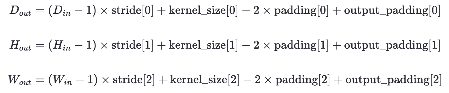
🟢 三维转置卷积:
nn.ConvTranspose3d用于视频、医学图像等体积数据
- 输入形状:
(N, C_{in}, D_{in}, H_{in}, W_{in})- 输出深度、高度、宽度计算公式:
✅ 所有维度的核心思想一致:
无论是一维、二维还是三维,转置卷积的输出尺寸计算都遵循同样的逻辑结构:
输出尺寸 ≈ 输入尺寸 × stride + 卷积核大小 - 填充修正 + 输出填充
🔍 补充说明几个关键参数的作用:
参数 作用 stride控制输入元素之间插入多少额外空间(通常是零),从而决定输出放大倍数。 stride=2→ 插入一个零,输出约为两倍长kernel_size决定卷积核大小,影响输出的偏移量 padding控制边缘裁剪/保留,通常用来对齐输入输出尺寸 output_padding额外添加在输出一侧的小偏移,用于微调输出尺寸(仅当 stride > 1 时有效)


nn.ConvTranspose1d是一维转置卷积层,也称为反卷积层,常用于上采样操作。参数
in_channels: 输入信号的通道数。out_channels: 输出信号的通道数。kernel_size: 转置卷积核的大小。stride: 转置卷积步长,默认为1。padding: 填充模式,默认为0。output_padding: 输出填充模式,默认为0。groups: 分组数量,默认为1。bias: 是否使用偏置项,默认为True。dilation: 空洞率,默认为1。
import torch
import torch.nn as nn

class ConvTranspose1DExample(nn.Module):
    def __init__(self):
        super(ConvTranspose1DExample, self).__init__()
        self.convtranspose1d = nn.ConvTranspose1d(in_channels=3, out_channels=6, kernel_size=5)

    def forward(self, x):
        return self.convtranspose1d(x)

# 创建一个输入张量,形状为 (batch_size, in_channels, length)
input_tensor = torch.randn(1, 3, 10)
model = ConvTranspose1DExample()
output = model(input_tensor)
print(output.shape) # 输出形状应为 (1, 6, 14)2.2.5、nn.ConvTranspose2d
nn.ConvTranspose2d是二维转置卷积层,也称为反卷积层,常用于上采样操作。参数
in_channels: 输入图像的通道数。out_channels: 输出图像的通道数。kernel_size: 转置卷积核的大小(可以是整数或元组)。stride: 转置卷积步长,默认为1。padding: 填充模式,默认为0。output_padding: 输出填充模式,默认为0。groups: 分组数量,默认为1。bias: 是否使用偏置项,默认为True。dilation: 空洞率,默认为1。
import torch
import torch.nn as nn

class ConvTranspose2DExample(nn.Module):
    def __init__(self):
        super(ConvTranspose2DExample, self).__init__()
        self.convtranspose2d = nn.ConvTranspose2d(in_channels=3, out_channels=6, kernel_size=(5, 5))

    def forward(self, x):
        return self.convtranspose2d(x)

# 创建一个输入张量,形状为 (batch_size, in_channels, height, width)
input_tensor = torch.randn(1, 3, 32, 32)
model = ConvTranspose2DExample()
output = model(input_tensor)
print(output.shape) # 输出形状应为 (1, 6, 36, 36)2.2.6、nn.ConvTranspose3d
nn.ConvTranspose3d是三维转置卷积层,也称为反卷积层,常用于上采样操作。参数
in_channels: 输入体积的通道数。out_channels: 输出体积的通道数。kernel_size: 转置卷积核的大小(可以是整数或元组)。stride: 转置卷积步长,默认为1。padding: 填充模式,默认为0。output_padding: 输出填充模式,默认为0。groups: 分组数量,默认为1。bias: 是否使用偏置项,默认为True。dilation: 空洞率,默认为1。
import torch
import torch.nn as nn

class ConvTranspose3DExample(nn.Module):
    def __init__(self):
        super(ConvTranspose3DExample, self).__init__()
        self.convtranspose3d = nn.ConvTranspose3d(in_channels=3, out_channels=6, kernel_size=(3, 3, 3))

    def forward(self, x):
        return self.convtranspose3d(x)

# 创建一个输入张量,形状为 (batch_size, in_channels, depth, height, width)
input_tensor = torch.randn(1, 3, 16, 16, 16)
model = ConvTranspose3DExample()
output = model(input_tensor)
print(output.shape)  # 输出形状应为 (1, 6, 18, 18, 18)
2.3、归一化层
层归一化(Layer Normalization, LN)的作用是通过对每个样本的所有特征维度进行标准化(均值为0,方差为1),再通过可学习的缩放(γγ)和平移(ββ)参数恢复表达能力,从而加速训练、缓解梯度消失/爆炸问题,并减少对批次大小的依赖。
2.3.1 nn.BatchNorm1d
nn.BatchNorm1d是一维批量归一化层,常用于处理一维信号数据。参数
num_features: 输入特征的数量。eps: 为数值稳定性添加的小值,默认为1e-5。momentum: 动态均值和方差计算中的动量项,默认为0.1。affine: 是否使用可学习的参数γ和β进行仿射变换,默认为True。track_running_stats: 是否跟踪动态统计信息,默认为True。
import torch
import torch.nn as nn

class BatchNorm1DExample(nn.Module):
    def __init__(self):
        super(BatchNorm1DExample, self).__init__()
        self.bn1d = nn.BatchNorm1d(num_features=6)

    def forward(self, x):
        return self.bn1d(x)

# 创建一个输入张量,形状为 (batch_size, num_features, length)
input_tensor = torch.randn(10, 6, 10)
model = BatchNorm1DExample()
output = model(input_tensor)
print(output.shape)  # 输出形状应为 (10, 6, 10)
2.3.2 nn.BatchNorm2d
nn.BatchNorm2d是二维批量归一化层,常用于图像处理任务。参数
num_features: 输入特征的数量(即通道数)。eps: 为数值稳定性添加的小值,默认为1e-5。momentum: 动态均值和方差计算中的动量项,默认为0.1。affine: 是否使用可学习的参数γ和β进行仿射变换,默认为True。track_running_stats: 是否跟踪动态统计信息,默认为True。
import torch
import torch.nn as nn

class BatchNorm2DExample(nn.Module):
    def __init__(self):
        super(BatchNorm2DExample, self).__init__()
        self.bn2d = nn.BatchNorm2d(num_features=6)

    def forward(self, x):
        return self.bn2d(x)

# 创建一个输入张量,形状为 (batch_size, num_features, height, width)
input_tensor = torch.randn(10, 6, 32, 32)
model = BatchNorm2DExample()
output = model(input_tensor)
print(output.shape)  # 输出形状应为 (10, 6, 32, 32)
2.3.3 nn.BatchNorm3d
nn.BatchNorm3d是三维批量归一化层,常用于视频处理或其他三维数据处理任务。参数
num_features: 输入特征的数量(即通道数)。eps: 为数值稳定性添加的小值,默认为1e-5。momentum: 动态均值和方差计算中的动量项,默认为0.1。affine: 是否使用可学习的参数γ和β进行仿射变换,默认为True。track_running_stats: 是否跟踪动态统计信息,默认为True。
import torch
import torch.nn as nn

class BatchNorm3DExample(nn.Module):
    def __init__(self):
        super(BatchNorm3DExample, self).__init__()
        self.bn3d = nn.BatchNorm3d(num_features=6)

    def forward(self, x):
        return self.bn3d(x)

# 创建一个输入张量,形状为 (batch_size, num_features, depth, height, width)
input_tensor = torch.randn(10, 6, 16, 16, 16)
model = BatchNorm3DExample()
output = model(input_tensor)
print(output.shape)  # 输出形状应为 (10, 6, 16, 16, 16)
2.3.4 nn.LayerNorm
nn.LayerNorm是层归一化层,对每个样本的所有特征维度进行归一化。参数
normalized_shape: 需要归一化的维度大小。eps: 为数值稳定性添加的小值,默认为1e-5。elementwise_affine: 是否使用可学习的参数γ和β进行仿射变换,默认为True。
import torch
import torch.nn as nn

class LayerNormExample(nn.Module):
    def __init__(self):
        super(LayerNormExample, self).__init__()
        self.ln = nn.LayerNorm(normalized_shape=(6, 10))

    def forward(self, x):
        return self.ln(x)

# 创建一个输入张量,形状为 (batch_size, num_features, length)
input_tensor = torch.randn(10, 6, 10)
model = LayerNormExample()
output = model(input_tensor)
print(output.shape)  # 输出形状应为 (10, 6, 10)
2.3.5 nn.InstanceNorm1d
nn.InstanceNorm1d是一维实例归一化层,对每个样本的所有通道进行归一化。参数
num_features: 输入特征的数量(即通道数)。eps: 为数值稳定性添加的小值,默认为1e-5。momentum: 动态均值和方差计算中的动量项,默认为0.1。affine: 是否使用可学习的参数γ和β进行仿射变换,默认为False。track_running_stats: 是否跟踪动态统计信息,默认为False。
import torch
import torch.nn as nn

class InstanceNorm1DExample(nn.Module):
    def __init__(self):
        super(InstanceNorm1DExample, self).__init__()
        self.in1d = nn.InstanceNorm1d(num_features=6, affine=True)

    def forward(self, x):
        return self.in1d(x)

# 创建一个输入张量,形状为 (batch_size, num_features, length)
input_tensor = torch.randn(10, 6, 10)
model = InstanceNorm1DExample()
output = model(input_tensor)
print(output.shape)  # 输出形状应为 (10, 6, 10)
2.3.6 nn.InstanceNorm2d
nn.InstanceNorm2d 是二维实例归一化层,对每个样本的所有通道进行归一化。
参数
num_features: 输入特征的数量(即通道数)。eps: 为数值稳定性添加的小值,默认为1e-5。momentum: 动态均值和方差计算中的动量项,默认为0.1。affine: 是否使用可学习的参数γ和β进行仿射变换,默认为False。track_running_stats: 是否跟踪动态统计信息,默认为False。
import torch
import torch.nn as nn

class InstanceNorm2DExample(nn.Module):
    def __init__(self):
        super(InstanceNorm2DExample, self).__init__()
        self.in2d = nn.InstanceNorm2d(num_features=6, affine=True)

    def forward(self, x):
        return self.in2d(x)

# 创建一个输入张量,形状为 (batch_size, num_features, height, width)
input_tensor = torch.randn(10, 6, 32, 32)
model = InstanceNorm2DExample()
output = model(input_tensor)
print(output.shape)  # 输出形状应为 (10, 6, 32, 32)
2.3.7 nn.InstanceNorm3d
nn.InstanceNorm3d 是三维实例归一化层,对每个样本的所有通道进行归一化。
参数
num_features: 输入特征的数量(即通道数)。eps: 为数值稳定性添加的小值,默认为1e-5。momentum: 动态均值和方差计算中的动量项,默认为0.1。affine: 是否使用可学习的参数γ和β进行仿射变换,默认为False。track_running_stats: 是否跟踪动态统计信息,默认为False。
import torch
import torch.nn as nn

class InstanceNorm3DExample(nn.Module):
    def __init__(self):
        super(InstanceNorm3DExample, self).__init__()
        self.in3d = nn.InstanceNorm3d(num_features=6, affine=True)

    def forward(self, x):
        return self.in3d(x)

# 创建一个输入张量,形状为 (batch_size, num_features, depth, height, width)
input_tensor = torch.randn(10, 6, 16, 16, 16)
model = InstanceNorm3DExample()
output = model(input_tensor)
print(output.shape)  # 输出形状应为 (10, 6, 16, 16, 16)
2.3.8 nn.GroupNorm
nn.GroupNorm是组归一化层,将特征分成若干组并对每组进行归一化。参数
num_groups: 特征维度分割成的组数。num_channels: 输入特征的数量(即通道数)。eps: 为数值稳定性添加的小值,默认为1e-5。affine: 是否使用可学习的参数γ和β进行仿射变换,默认为True。
import torch
import torch.nn as nn

class GroupNormExample(nn.Module):
    def __init__(self):
        super(GroupNormExample, self).__init__()
        self.gn = nn.GroupNorm(num_groups=3, num_channels=6)

    def forward(self, x):
        return self.gn(x)

# 创建一个输入张量,形状为 (batch_size, num_channels, height, width)
input_tensor = torch.randn(10, 6, 32, 32)
model = GroupNormExample()
output = model(input_tensor)
print(output.shape)  # 输出形状应为 (10, 6, 32, 32)
2.4、激活函数
2.4.1 nn.ReLU
nn.ReLU是线性整流单元(Rectified Linear Unit),输出为max(0, x)。参数
inplace: 是否进行原地操作,默认为False。
import torch
import torch.nn as nn

class ReLUExample(nn.Module):
    def __init__(self):
        super(ReLUExample, self).__init__()
        self.relu = nn.ReLU()

    def forward(self, x):
        return self.relu(x)

# 创建一个输入张量
input_tensor = torch.tensor([-1.0, 0.0, 1.0, 2.0], requires_grad=True)
model = ReLUExample()
output = model(input_tensor)
print(output)  # 输出应为 tensor([0., 0., 1., 2.])
2.4.2 nn.ReLU6
nn.ReLU6类似于nn.ReLU,但输出范围限制在[0, 6]。参数
inplace: 是否进行原地操作,默认为False。
import torch
import torch.nn as nn

class ReLU6Example(nn.Module):
    def __init__(self):
        super(ReLU6Example, self).__init__()
        self.relu6 = nn.ReLU6()

    def forward(self, x):
        return self.relu6(x)

# 创建一个输入张量
input_tensor = torch.tensor([-1.0, 0.0, 1.0, 2.0, 7.0], requires_grad=True)
model = ReLU6Example()
output = model(input_tensor)
print(output)  # 输出应为 tensor([0., 0., 1., 2., 6.])
2.4.3 nn.Sigmoid
nn.Sigmoid 将输入映射到 (0, 1) 区间,公式为 sigmoid(x) = 1 / (1 + exp(-x))。
import torch
import torch.nn as nn

class SigmoidExample(nn.Module):
    def __init__(self):
        super(SigmoidExample, self).__init__()
        self.sigmoid = nn.Sigmoid()

    def forward(self, x):
        return self.sigmoid(x)

# 创建一个输入张量
input_tensor = torch.tensor([-1.0, 0.0, 1.0], requires_grad=True)
model = SigmoidExample()
output = model(input_tensor)
print(output)  # 输出应为 tensor([0.2689, 0.5000, 0.7311])
2.4.4 nn.Tanh
nn.Tanh 将输入映射到 (-1, 1) 区间,公式为 tanh(x) = (exp(x) - exp(-x)) / (exp(x) + exp(-x))。
import torch
import torch.nn as nn

class TanhExample(nn.Module):
    def __init__(self):
        super(TanhExample, self).__init__()
        self.tanh = nn.Tanh()

    def forward(self, x):
        return self.tanh(x)

# 创建一个输入张量
input_tensor = torch.tensor([-1.0, 0.0, 1.0], requires_grad=True)
model = TanhExample()
output = model(input_tensor)
print(output)  # 输出应为 tensor([-0.7616,  0.0000,  0.7616])
2.4.5 nn.Softmax
nn.Softmax将输入转换为概率分布,公式为softmax(x_i) = exp(x_i) / sum(exp(x_j))。参数
dim: 指定应用 softmax 的维度。
import torch
import torch.nn as nn

class SoftmaxExample(nn.Module):
    def __init__(self):
        super(SoftmaxExample, self).__init__()
        self.softmax = nn.Softmax(dim=1)

    def forward(self, x):
        return self.softmax(x)

# 创建一个输入张量
input_tensor = torch.tensor([[1.0, 2.0, 3.0], [4.0, 5.0, 6.0]], requires_grad=True)
model = SoftmaxExample()
output = model(input_tensor)
print(output)  # 输出应为 tensor([[0.0900, 0.2447, 0.6652],
                             #         [0.0900, 0.2447, 0.6652]])
2.4.6 nn.Softmax2d
nn.Softmax2d 对二维空间上的每个像素位置应用 softmax 函数。
import torch
import torch.nn as nn

class Softmax2DExample(nn.Module):
    def __init__(self):
        super(Softmax2DExample, self).__init__()
        self.softmax2d = nn.Softmax2d()

    def forward(self, x):
        return self.softmax2d(x)

# 创建一个输入张量,形状为 (batch_size, channels, height, width)
input_tensor = torch.randn(1, 3, 2, 2)
model = Softmax2DExample()
output = model(input_tensor)
print(output.shape)  # 输出形状应为 (1, 3, 2, 2)
2.4.7 nn.LogSoftmax
nn.LogSoftmax计算 softmax 的对数,公式为log_softmax(x_i) = log(exp(x_i) / sum(exp(x_j)))。参数
dim: 指定应用 log_softmax 的维度。
import torch
import torch.nn as nn

class LogSoftmaxExample(nn.Module):
    def __init__(self):
        super(LogSoftmaxExample, self).__init__()
        self.logsoftmax = nn.LogSoftmax(dim=1)

    def forward(self, x):
        return self.logsoftmax(x)

# 创建一个输入张量
input_tensor = torch.tensor([[1.0, 2.0, 3.0], [4.0, 5.0, 6.0]], requires_grad=True)
model = LogSoftmaxExample()
output = model(input_tensor)
print(output)  # 输出应为 tensor([[-2.4076, -1.4076, -0.4076],
                                #         [-2.4076, -1.4076, -0.4076]])
2.4.8 nn.ELU
nn.ELU指数线性单位,公式为elu(x) = max(0, x) + min(0, alpha * (exp(x) - 1))。参数
alpha: 控制负斜率部分的参数,默认为1.0。inplace: 是否进行原地操作,默认为False。
import torch
import torch.nn as nn

class ELUExample(nn.Module):
    def __init__(self):
        super(ELUExample, self).__init__()
        self.elu = nn.ELU(alpha=1.0)

    def forward(self, x):
        return self.elu(x)

# 创建一个输入张量
input_tensor = torch.tensor([-1.0, 0.0, 1.0], requires_grad=True)
model = ELUExample()
output = model(input_tensor)
print(output)  # 输出应为 tensor([-0.6321,  0.0000,  1.0000])
2.4.9 nn.LeakyReLU
nn.LeakyReLU泄漏线性整流单元,公式为leaky_relu(x) = max(0, x) + negative_slope * min(0, x)。参数
negative_slope: 负斜率部分的系数,默认为0.01。inplace: 是否进行原地操作,默认为False。
import torch
import torch.nn as nn

class LeakyReLUExample(nn.Module):
    def __init__(self):
        super(LeakyReLUExample, self).__init__()
        self.leakyrelu = nn.LeakyReLU(negative_slope=0.01)

    def forward(self, x):
        return self.leakyrelu(x)

# 创建一个输入张量
input_tensor = torch.tensor([-1.0, 0.0, 1.0], requires_grad=True)
model = LeakyReLUExample()
output = model(input_tensor)
print(output)  # 输出应为 tensor([-0.0100,  0.0000,  1.0000])
2.4.10 nn.PReLU
nn.PReLU可学习的泄漏线性整流单元,负斜率是一个可学习的参数。参数
num_parameters: 学习的负斜率的数量,如果为1,则所有通道共享相同的负斜率;否则,每个通道有自己的负斜率。init: 初始值,默认为0.25。
import torch
import torch.nn as nn

class PReLUExample(nn.Module):
    def __init__(self):
        super(PReLUExample, self).__init__()
        self.prelu = nn.PReLU(num_parameters=1, init=0.25)

    def forward(self, x):
        return self.prelu(x)

# 创建一个输入张量
input_tensor = torch.tensor([-1.0, 0.0, 1.0], requires_grad=True)
model = PReLUExample()
output = model(input_tensor)
print(output)  # 输出应为 tensor([-0.2500,  0.0000,  1.0000])
2.4.11 nn.SELU
nn.SELU自然指数线性单元,公式为selu(x) = scale * elu(x, alpha, 1.0)。参数
inplace: 是否进行原地操作,默认为False。
import torch
import torch.nn as nn

class SELUExample(nn.Module):
    def __init__(self):
        super(SELUExample, self).__init__()
        self.selu = nn.SELU()

    def forward(self, x):
        return self.selu(x)

# 创建一个输入张量
input_tensor = torch.tensor([-1.0, 0.0, 1.0], requires_grad=True)
model = SELUExample()
output = model(input_tensor)
print(output)  # 输出应为 tensor([-1.1113,  0.0000,  1.0507])
2.4.12 nn.GELU
nn.GELU高斯误差线性单元,公式为gelu(x) = 0.5 * x * (1 + tanh(sqrt(2/pi) * (x + 0.044715 * x^3)))。参数
approximate: 使用近似版本,默认为'none'。
import torch
import torch.nn as nn

class GELUExample(nn.Module):
    def __init__(self):
        super(GELUExample, self).__init__()
        self.gelu = nn.GELU(approximate='none')

    def forward(self, x):
        return self.gelu(x)

# 创建一个输入张量
input_tensor = torch.tensor([-1.0, 0.0, 1.0], requires_grad=True)
model = GELUExample()
output = model(input_tensor)
print(output)  # 输出应为 tensor([-0.1587,  0.0000,  0.8412])
2.5、池化层
2.5.1 nn.MaxPool1d
nn.MaxPool1d是一维最大池化层,常用于处理一维信号数据。参数
kernel_size: 池化窗口的大小。stride: 池化窗口的步长,默认为kernel_size。padding: 输入两侧填充的元素数量,默认为0。dilation: 控制窗口中元素之间的间距,默认为1。return_indices: 是否返回最大值索引,默认为False。ceil_mode: 如果为True,则向上取整计算输出形状,默认为False。
import torch
import torch.nn as nn

class MaxPool1DExample(nn.Module):
    def __init__(self):
        super(MaxPool1DExample, self).__init__()
        self.maxpool1d = nn.MaxPool1d(kernel_size=3, stride=2)

    def forward(self, x):
        return self.maxpool1d(x)

# 创建一个输入张量,形状为 (batch_size, channels, length)
input_tensor = torch.tensor([[[1.0, 2.0, 3.0, 4.0, 5.0, 6.0]]], requires_grad=True)
model = MaxPool1DExample()
output = model(input_tensor)
print(output)  # 输出应为 tensor([[[2., 4., 6.]]])
2.5.2 nn.MaxPool2d
nn.MaxPool2d是二维最大池化层,常用于图像处理任务。参数
kernel_size: 池化窗口的大小(可以是整数或元组)。stride: 池化窗口的步长,默认为kernel_size。padding: 输入两侧填充的元素数量,默认为0。dilation: 控制窗口中元素之间的间距,默认为1。return_indices: 是否返回最大值索引,默认为False。ceil_mode: 如果为True,则向上取整计算输出形状,默认为False。
import torch
import torch.nn as nn

class MaxPool2DExample(nn.Module):
    def __init__(self):
        super(MaxPool2DExample, self).__init__()
        self.maxpool2d = nn.MaxPool2d(kernel_size=(2, 2), stride=2)

    def forward(self, x):
        return self.maxpool2d(x)

# 创建一个输入张量,形状为 (batch_size, channels, height, width)
input_tensor = torch.tensor([[[[1.0, 2.0, 3.0, 4.0],
                              [5.0, 6.0, 7.0, 8.0],
                              [9.0, 10.0, 11.0, 12.0],
                              [13.0, 14.0, 15.0, 16.0]]]], requires_grad=True)
model = MaxPool2DExample()
output = model(input_tensor)
print(output)  # 输出应为 tensor([[[[ 6.,  8.],
                                 #          [14., 16.]]]])
2.5.3 nn.MaxPool3d
nn.MaxPool3d是三维最大池化层,常用于视频处理或其他三维数据处理任务。参数
kernel_size: 池化窗口的大小(可以是整数或元组)。stride: 池化窗口的步长,默认为kernel_size。padding: 输入两侧填充的元素数量,默认为0。dilation: 控制窗口中元素之间的间距,默认为1。return_indices: 是否返回最大值索引,默认为False。ceil_mode: 如果为True,则向上取整计算输出形状,默认为False。
import torch
import torch.nn as nn

class MaxPool3DExample(nn.Module):
    def __init__(self):
        super(MaxPool3DExample, self).__init__()
        self.maxpool3d = nn.MaxPool3d(kernel_size=(2, 2, 2), stride=2)

    def forward(self, x):
        return self.maxpool3d(x)

# 创建一个输入张量,形状为 (batch_size, channels, depth, height, width)
input_tensor = torch.tensor([[[[[ 1.0,  2.0,  3.0,  4.0],
                               [ 5.0,  6.0,  7.0,  8.0],
                               [ 9.0, 10.0, 11.0, 12.0],
                               [13.0, 14.0, 15.0, 16.0]],
                              [[17.0, 18.0, 19.0, 20.0],
                               [21.0, 22.0, 23.0, 24.0],
                               [25.0, 26.0, 27.0, 28.0],
                               [29.0, 30.0, 31.0, 32.0]],
                              [[33.0, 34.0, 35.0, 36.0],
                               [37.0, 38.0, 39.0, 40.0],
                               [41.0, 42.0, 43.0, 44.0],
                               [45.0, 46.0, 47.0, 48.0]],
                              [[49.0, 50.0, 51.0, 52.0],
                               [53.0, 54.0, 55.0, 56.0],
                               [57.0, 58.0, 59.0, 60.0],
                               [61.0, 62.0, 63.0, 64.0]]]]], requires_grad=True)
model = MaxPool3DExample()
output = model(input_tensor)
print(output)  # 输出应为 tensor([[[[[22., 24.],
                                    #            [30., 32.]],
                                   #           [[38., 40.],
                                    #            [46., 48.]]]])
2.5.4 nn.AvgPool1d
nn.AvgPool1d是一维平均池化层,常用于处理一维信号数据。参数
kernel_size: 池化窗口的大小。stride: 池化窗口的步长,默认为kernel_size。padding: 输入两侧填充的元素数量,默认为0。ceil_mode: 如果为True,则向上取整计算输出形状,默认为False。count_include_pad: 如果为True,则在计算平均时包括填充的零,默认为True。
import torch
import torch.nn as nn

class AvgPool1DExample(nn.Module):
    def __init__(self):
        super(AvgPool1DExample, self).__init__()
        self.avgpool1d = nn.AvgPool1d(kernel_size=3, stride=2)

    def forward(self, x):
        return self.avgpool1d(x)

# 创建一个输入张量,形状为 (batch_size, channels, length)
input_tensor = torch.tensor([[[1.0, 2.0, 3.0, 4.0, 5.0, 6.0]]], requires_grad=True)
model = AvgPool1DExample()
output = model(input_tensor)
print(output)  # 输出应为 tensor([[[2., 4., 5.]]])
2.5.5 nn.AvgPool2d
nn.AvgPool2d是二维平均池化层,常用于图像处理任务。参数
kernel_size: 池化窗口的大小(可以是整数或元组)。stride: 池化窗口的步长,默认为kernel_size。padding: 输入两侧填充的元素数量,默认为0。ceil_mode: 如果为True,则向上取整计算输出形状,默认为False。count_include_pad: 如果为True,则在计算平均时包括填充的零,默认为True。
import torch
import torch.nn as nn

class AvgPool2DExample(nn.Module):
    def __init__(self):
        super(AvgPool2DExample, self).__init__()
        self.avgpool2d = nn.AvgPool2d(kernel_size=(2, 2), stride=2)

    def forward(self, x):
        return self.avgpool2d(x)

# 创建一个输入张量,形状为 (batch_size, channels, height, width)
input_tensor = torch.tensor([[[[1.0, 2.0, 3.0, 4.0],
                              [5.0, 6.0, 7.0, 8.0],
                              [9.0, 10.0, 11.0, 12.0],
                              [13.0, 14.0, 15.0, 16.0]]]], requires_grad=True)
model = AvgPool2DExample()
output = model(input_tensor)
print(output)  # 输出应为 tensor([[[[ 3.5,  5.5],
                                  #          [11.5, 13.5]]]])
2.5.6 nn.AvgPool3d
nn.AvgPool3d是三维平均池化层,常用于视频处理或其他三维数据处理任务。参数
kernel_size: 池化窗口的大小(可以是整数或元组)。stride: 池化窗口的步长,默认为kernel_size。padding: 输入两侧填充的元素数量,默认为0。ceil_mode: 如果为True,则向上取整计算输出形状,默认为False。count_include_pad: 如果为True,则在计算平均时包括填充的零,默认为True。
import torch
import torch.nn as nn

class AvgPool3DExample(nn.Module):
    def __init__(self):
        super(AvgPool3DExample, self).__init__()
        self.avgpool3d = nn.AvgPool3d(kernel_size=(2, 2, 2), stride=2)

    def forward(self, x):
        return self.avgpool3d(x)

# 创建一个输入张量,形状为 (batch_size, channels, depth, height, width)
input_tensor = torch.tensor([[[[[ 1.0,  2.0,  3.0,  4.0],
                               [ 5.0,  6.0,  7.0,  8.0],
                               [ 9.0, 10.0, 11.0, 12.0],
                               [13.0, 14.0, 15.0, 16.0]],
                              [[17.0, 18.0, 19.0, 20.0],
                               [21.0, 22.0, 23.0, 24.0],
                               [25.0, 26.0, 27.0, 28.0],
                               [29.0, 30.0, 31.0, 32.0]],
                              [[33.0, 34.0, 35.0, 36.0],
                               [37.0, 38.0, 39.0, 40.0],
                               [41.0, 42.0, 43.0, 44.0],
                               [45.0, 46.0, 47.0, 48.0]],
                              [[49.0, 50.0, 51.0, 52.0],
                               [53.0, 54.0, 55.0, 56.0],
                               [57.0, 58.0, 59.0, 60.0],
                               [61.0, 62.0, 63.0, 64.0]]]]], requires_grad=True)
model = AvgPool3DExample()
output = model(input_tensor)
print(output)  # 输出应为 tensor([[[[[22., 24.],
                                     #             [30., 32.]],
                                    #            [[38., 40.],
                                     #             [46., 48.]]]])
2.5.7 nn.AdaptiveMaxPool1d
nn.AdaptiveMaxPool1d是自适应的一维最大池化层,输出尺寸由用户指定。参数
output_size: 目标输出尺寸。
import torch
import torch.nn as nn

class AdaptiveMaxPool1DExample(nn.Module):
    def __init__(self):
        super(AdaptiveMaxPool1DExample, self).__init__()
        self.adaptivemaxpool1d = nn.AdaptiveMaxPool1d(output_size=3)

    def forward(self, x):
        return self.adaptivemaxpool1d(x)

# 创建一个输入张量,形状为 (batch_size, channels, length)
input_tensor = torch.tensor([[[1.0, 2.0, 3.0, 4.0, 5.0, 6.0]]], requires_grad=True)
model = AdaptiveMaxPool1DExample()
output = model(input_tensor)
print(output)  # 输出应为 tensor([[[4., 5., 6.]]])
2.5.8 nn.AdaptiveMaxPool2d
nn.AdaptiveMaxPool2d是自适应的二维最大池化层,输出尺寸由用户指定。参数
output_size: 目标输出尺寸(可以是整数或元组)。
import torch
import torch.nn as nn

class AdaptiveMaxPool2DExample(nn.Module):
    def __init__(self):
        super(AdaptiveMaxPool2DExample, self).__init__()
        self.adaptivemaxpool2d = nn.AdaptiveMaxPool2d(output_size=(2, 2))

    def forward(self, x):
        return self.adaptivemaxpool2d(x)

# 创建一个输入张量,形状为 (batch_size, channels, height, width)
input_tensor = torch.tensor([[[[1.0, 2.0, 3.0, 4.0],
                              [5.0, 6.0, 7.0, 8.0],
                              [9.0, 10.0, 11.0, 12.0],
                              [13.0, 14.0, 15.0, 16.0]]]], requires_grad=True)
model = AdaptiveMaxPool2DExample()
output = model(input_tensor)
print(output)  # 输出应为 tensor([[[[ 6.,  8.],
                                  #          [14., 16.]]]])
2.5.9 nn.AdaptiveMaxPool3d
nn.AdaptiveMaxPool3d是自适应的三维最大池化层,输出尺寸由用户指定。参数
output_size: 目标输出尺寸(可以是整数或元组)。
import torch
import torch.nn as nn

class AdaptiveMaxPool3DExample(nn.Module):
    def __init__(self):
        super(AdaptiveMaxPool3DExample, self).__init__()
        self.adaptivemaxpool3d = nn.AdaptiveMaxPool3d(output_size=(2, 2, 2))

    def forward(self, x):
        return self.adaptivemaxpool3d(x)

# 创建一个输入张量,形状为 (batch_size, channels, depth, height, width)
input_tensor = torch.tensor([[[[[ 1.0,  2.0,  3.0,  4.0],
                               [ 5.0,  6.0,  7.0,  8.0],
                               [ 9.0, 10.0, 11.0, 12.0],
                               [13.0, 14.0, 15.0, 16.0]],
                              [[17.0, 18.0, 19.0, 20.0],
                               [21.0, 22.0, 23.0, 24.0],
                               [25.0, 26.0, 27.0, 28.0],
                               [29.0, 30.0, 31.0, 32.0]],
                              [[33.0, 34.0, 35.0, 36.0],
                               [37.0, 38.0, 39.0, 40.0],
                               [41.0, 42.0, 43.0, 44.0],
                               [45.0, 46.0, 47.0, 48.0]],
                              [[49.0, 50.0, 51.0, 52.0],
                               [53.0, 54.0, 55.0, 56.0],
                               [57.0, 58.0, 59.0, 60.0],
                               [61.0, 62.0, 63.0, 64.0]]]]], requires_grad=True)
model = AdaptiveMaxPool3DExample()
output = model(input_tensor)
print(output)  # 输出应为 tensor([[[[[22., 24.],
                                     #              [30., 32.]],
                                    #             [[38., 40.],
                                     #              [46., 48.]]]])
2.5.10 nn.AdaptiveAvgPool1d
nn.AdaptiveAvgPool1d是自适应的一维平均池化层,输出尺寸由用户指定。参数
output_size: 目标输出尺寸。
import torch
import torch.nn as nn

class AdaptiveAvgPool1DExample(nn.Module):
    def __init__(self):
        super(AdaptiveAvgPool1DExample, self).__init__()
        self.adaptiveavgpool1d = nn.AdaptiveAvgPool1d(output_size=3)

    def forward(self, x):
        return self.adaptiveavgpool1d(x)

# 创建一个输入张量,形状为 (batch_size, channels, length)
input_tensor = torch.tensor([[[1.0, 2.0, 3.0, 4.0, 5.0, 6.0]]], requires_grad=True)
model = AdaptiveAvgPool1DExample()
output = model(input_tensor)
print(output)  # 输出应为 tensor([[[2., 4., 5.]]])
2.5.11 nn.AdaptiveAvgPool2d
nn.AdaptiveAvgPool2d是自适应的二维平均池化层,输出尺寸由用户指定。参数
output_size: 目标输出尺寸(可以是整数或元组)。
import torch
import torch.nn as nn

class AdaptiveAvgPool2DExample(nn.Module):
    def __init__(self):
        super(AdaptiveAvgPool2DExample, self).__init__()
        self.adaptiveavgpool2d = nn.AdaptiveAvgPool2d(output_size=(2, 2))

    def forward(self, x):
        return self.adaptiveavgpool2d(x)

# 创建一个输入张量,形状为 (batch_size, channels, height, width)
input_tensor = torch.tensor([[[[1.0, 2.0, 3.0, 4.0],
                              [5.0, 6.0, 7.0, 8.0],
                              [9.0, 10.0, 11.0, 12.0],
                              [13.0, 14.0, 15.0, 16.0]]]], requires_grad=True)
model = AdaptiveAvgPool2DExample()
output = model(input_tensor)
print(output)  # 输出应为 tensor([[[[ 3.5,  5.5],
                                  #          [11.5, 13.5]]]])
2.5.12 nn.AdaptiveAvgPool3d
nn.AdaptiveAvgPool3d是自适应的三维平均池化层,输出尺寸由用户指定。参数
output_size: 目标输出尺寸(可以是整数或元组)。
import torch
import torch.nn as nn

class AdaptiveAvgPool3DExample(nn.Module):
    def __init__(self):
        super(AdaptiveAvgPool3DExample, self).__init__()
        self.adaptiveavgpool3d = nn.AdaptiveAvgPool3d(output_size=(2, 2, 2))

    def forward(self, x):
        return self.adaptiveavgpool3d(x)

# 创建一个输入张量,形状为 (batch_size, channels, depth, height, width)
input_tensor = torch.tensor([[[[[ 1.0,  2.0,  3.0,  4.0],
                               [ 5.0,  6.0,  7.0,  8.0],
                               [ 9.0, 10.0, 11.0, 12.0],
                               [13.0, 14.0, 15.0, 16.0]],
                              [[17.0, 18.0, 19.0, 20.0],
                               [21.0, 22.0, 23.0, 24.0],
                               [25.0, 26.0, 27.0, 28.0],
                               [29.0, 30.0, 31.0, 32.0]],
                              [[33.0, 34.0, 35.0, 36.0],
                               [37.0, 38.0, 39.0, 40.0],
                               [41.0, 42.0, 43.0, 44.0],
                               [45.0, 46.0, 47.0, 48.0]],
                              [[49.0, 50.0, 51.0, 52.0],
                               [53.0, 54.0, 55.0, 56.0],
                               [57.0, 58.0, 59.0, 60.0],
                               [61.0, 62.0, 63.0, 64.0]]]]], requires_grad=True)
model = AdaptiveAvgPool3DExample()
output = model(input_tensor)
print(output)  # 输出应为 tensor([[[[[22., 24.],
                                     #              [30., 32.]],
                                    #             [[38., 40.],
# [46., 48.]]]])2.6、正则化与降维层
2.6.1 nn.Dropout
nn.Dropout是一种在训练过程中随机丢弃部分神经元的技术,用于防止过拟合。参数
p: 每个元素被丢弃的概率,默认为0.5。inplace: 是否进行原地操作,默认为False。
import torch
import torch.nn as nn

class DropoutExample(nn.Module):
    def __init__(self):
        super(DropoutExample, self).__init__()
        self.dropout = nn.Dropout(p=0.5)

    def forward(self, x):
        return self.dropout(x)

# 创建一个输入张量
input_tensor = torch.tensor([[1.0, 2.0, 3.0, 4.0]], requires_grad=True)
model = DropoutExample()
output = model(input_tensor)
print(output)  # 输出应为 tensor([[2., 0., 6., 0.]]) 或其他随机结果
2.6.2 nn.Dropout2d
nn.Dropout2d类似于nn.Dropout,但应用于二维数据(如图像),按通道丢弃整个特征图。参数
p: 每个特征图被丢弃的概率,默认为0.5。inplace: 是否进行原地操作,默认为False。
import torch
import torch.nn as nn

class Dropout2DExample(nn.Module):
    def __init__(self):
        super(Dropout2DExample, self).__init__()
        self.dropout2d = nn.Dropout2d(p=0.5)

    def forward(self, x):
        return self.dropout2d(x)

# 创建一个输入张量,形状为 (batch_size, channels, height, width)
input_tensor = torch.tensor([[[[1.0, 2.0],
                              [3.0, 4.0]],
                             [[5.0, 6.0],
                              [7.0, 8.0]]]], requires_grad=True)
model = Dropout2DExample()
output = model(input_tensor)
print(output)  # 输出应为 tensor([[[[2., 0.],
                                  #          [6., 0.]],
                                 #         [[0., 0.],
                                  #          [0., 0.]]]) 或其他随机结果
2.6.3 nn.Dropout3d
nn.Dropout3d类似于nn.Dropout2d,但应用于三维数据(如视频),按通道丢弃整个体素图。参数
p: 每个体素图被丢弃的概率,默认为0.5。inplace: 是否进行原地操作,默认为False。
import torch
import torch.nn as nn

class Dropout3DExample(nn.Module):
    def __init__(self):
        super(Dropout3DExample, self).__init__()
        self.dropout3d = nn.Dropout3d(p=0.5)

    def forward(self, x):
        return self.dropout3d(x)

# 创建一个输入张量,形状为 (batch_size, channels, depth, height, width)
input_tensor = torch.tensor([[[[[ 1.0,  2.0],
                               [ 3.0,  4.0]],
                              [[ 5.0,  6.0],
                               [ 7.0,  8.0]]],
                             [[[ 9.0, 10.0],
                               [11.0, 12.0]],
                              [[13.0, 14.0],
                               [15.0, 16.0]]]]], requires_grad=True)
model = Dropout3DExample()
output = model(input_tensor)
print(output)  # 输出应为 tensor([[[[[ 2.,  0.],
                                     #              [ 6.,  0.]],
                                    #             [[10.,  0.],
                                     #              [14.,  0.]]],
                                   #            [[[18.,  0.],
                                     #              [22.,  0.]],
                                    #             [[26.,  0.],
                                     #              [30.,  0.]]]]) 或其他随机结果
2.6.4 nn.AlphaDropout
nn.AlphaDropout是一种特殊的 dropout 技术,适用于自归一化激活函数(如 SELU),保持输出的均值和方差不变。参数
p: 每个元素被丢弃的概率,默认为0.5。
import torch
import torch.nn as nn

class AlphaDropoutExample(nn.Module):
    def __init__(self):
        super(AlphaDropoutExample, self).__init__()
        self.alphadropout = nn.AlphaDropout(p=0.5)

    def forward(self, x):
        return self.alphadropout(x)

# 创建一个输入张量
input_tensor = torch.tensor([[1.0, 2.0, 3.0, 4.0]], requires_grad=True)
model = AlphaDropoutExample()
output = model(input_tensor)
print(output) # 输出应为 tensor([[2., 0., 6., 0.]]) 或其他随机结果2.7、图像变换层
2.7.1 nn.Upsample
nn.Upsample是一个用于上采样的模块,可以通过多种方法(如最近邻插值、双线性插值等)来增加输入张量的空间尺寸。参数
size: 输出张量的目标大小。scale_factor: 相对于输入张量的缩放因子。mode: 上采样方法,可以是'nearest','linear','bilinear','bicubic','trilinear'等,默认为'nearest'。align_corners: 如果为True,则对齐角点,仅在'bilinear'和'bicubic'模式下有效,默认为None。
import torch
import torch.nn as nn

class UpsampleExample(nn.Module):
    def __init__(self, scale_factor, mode='bilinear'):
        super(UpsampleExample, self).__init__()
        self.upsample = nn.Upsample(scale_factor=scale_factor, mode=mode, align_corners=True if mode in ['bilinear', 'bicubic'] else None)

    def forward(self, x):
        return self.upsample(x)

# 创建一个输入张量,形状为 (batch_size, channels, height, width)
input_tensor = torch.randn(1, 3, 4, 4)  # batch_size=1, channels=3, height=4, width=4
model = UpsampleExample(scale_factor=2, mode='bilinear')
output = model(input_tensor)
print("Input shape:", input_tensor.shape)  # 输入应为 (1, 3, 4, 4)
print("Output shape:", output.shape)       # 输出应为 (1, 3, 8, 8)
2.7.2 nn.PixelShuffle
nn.PixelShuffle是一种用于将特征图中的像素重新排列的方法,常用于超分辨率任务。参数
upscale_factor: 上升比例因子,必须大于等于1。
import torch
import torch.nn as nn

class PixelShuffleExample(nn.Module):
    def __init__(self, upscale_factor):
        super(PixelShuffleExample, self).__init__()
        self.pixel_shuffle = nn.PixelShuffle(upscale_factor=upscale_factor)

    def forward(self, x):
        return self.pixel_shuffle(x)

# 创建一个输入张量,形状为 (batch_size, channels * upscale_factor^2, height, width)
input_tensor = torch.randn(1, 12, 4, 4)  # batch_size=1, channels=12, height=4, width=4
model = PixelShuffleExample(upscale_factor=2)
output = model(input_tensor)
print("Input shape:", input_tensor.shape)  # 输入应为 (1, 12, 4, 4)
print("Output shape:", output.shape)       # 输出应为 (1, 3, 8, 8)
2.7.3 nn.Fold
nn.Fold将滑动窗口内的元素折叠成固定形状的张量。参数
output_size: 输出张量的空间维度大小。kernel_size: 卷积核的大小。dilation: 控制卷积核中元素之间的间距,默认为1。padding: 输入两侧填充的元素数量,默认为0。stride: 卷积核移动的步长,默认为1。
import torch
import torch.nn as nn

class FoldExample(nn.Module):
    def __init__(self, output_size, kernel_size, dilation=1, padding=0, stride=1):
        super(FoldExample, self).__init__()
        self.fold = nn.Fold(output_size=output_size, kernel_size=kernel_size, dilation=dilation, padding=padding, stride=stride)

    def forward(self, x):
        return self.fold(x)

# 创建一个输入张量,形状为 (batch_size, channels * kernel_height * kernel_width, L)
input_tensor = torch.randn(1, 3 * 2 * 2, 9)  # batch_size=1, channels=3, kernel_height=2, kernel_width=2, L=9
model = FoldExample(output_size=(4, 4), kernel_size=(2, 2))
output = model(input_tensor)
print("Input shape:", input_tensor.shape)  # 输入应为 (1, 12, 9)
print("Output shape:", output.shape)       # 输出应为 (1, 3, 4, 4)
2.7.4 nn.Unfold
nn.Unfold将输入张量中的滑动窗口提取出来并展平。参数
kernel_size: 卷积核的大小。dilation: 控制卷积核中元素之间的间距,默认为1。padding: 输入两侧填充的元素数量,默认为0。stride: 卷积核移动的步长,默认为1。
import torch
import torch.nn as nn

class UnfoldExample(nn.Module):
    def __init__(self, kernel_size, dilation=1, padding=0, stride=1):
        super(UnfoldExample, self).__init__()
        self.unfold = nn.Unfold(kernel_size=kernel_size, dilation=dilation, padding=padding, stride=stride)

    def forward(self, x):
        return self.unfold(x)

# 创建一个输入张量,形状为 (batch_size, channels, height, width)
input_tensor = torch.randn(1, 3, 4, 4)  # batch_size=1, channels=3, height=4, width=4
model = UnfoldExample(kernel_size=(2, 2))
output = model(input_tensor)
print("Input shape:", input_tensor.shape)  # 输入应为 (1, 3, 4, 4)
print("Output shape:", output.shape) # 输出应为 (1, 12, 9)2.8、工具性模块
2.8.1 nn.Flatten
nn.Flatten是一个用于将输入张量展平为一维向量的模块。参数
start_dim: 开始展平的维度,默认为1。end_dim: 结束展平的维度,默认为-1。
import torch
import torch.nn as nn

class FlattenExample(nn.Module):
    def __init__(self, start_dim=1, end_dim=-1):
        super(FlattenExample, self).__init__()
        self.flatten = nn.Flatten(start_dim=start_dim, end_dim=end_dim)

    def forward(self, x):
        return self.flatten(x)

# 创建一个输入张量,形状为 (batch_size, channels, height, width)
input_tensor = torch.randn(1, 3, 4, 4)  # batch_size=1, channels=3, height=4, width=4
model = FlattenExample()
output = model(input_tensor)
print("Input shape:", input_tensor.shape)  # 输入应为 (1, 3, 4, 4)
print("Output shape:", output.shape)       # 输出应为 (1, 48)
2.8.2 nn.Identity
nn.Identity是一个简单的恒等变换层,直接返回输入张量而不进行任何操作。参数
- 无参数。
import torch
import torch.nn as nn

class IdentityExample(nn.Module):
    def __init__(self):
        super(IdentityExample, self).__init__()
        self.identity = nn.Identity()

    def forward(self, x):
        return self.identity(x)

# 创建一个输入张量
input_tensor = torch.randn(1, 3, 4, 4)  # batch_size=1, channels=3, height=4, width=4
model = IdentityExample()
output = model(input_tensor)
print("Input shape:", input_tensor.shape)  # 输入应为 (1, 3, 4, 4)
print("Output shape:", output.shape)       # 输出应为 (1, 3, 4, 4)
2.8.3 nn.Pad
nn.Pad是一个用于对输入张量进行填充的模块。参数
padding: 填充的大小,可以是一个整数或元组。mode: 填充模式,可以是'constant','reflect','replicate','circular'等,默认为'constant'。value: 如果mode为'constant',则指定填充值,默认为0。
import torch
import torch.nn as nn

class PadExample(nn.Module):
    def __init__(self, padding, mode='constant', value=0):
        super(PadExample, self).__init__()
        self.pad = nn.ReflectionPad2d(padding=padding)  # 使用反射填充作为示例

    def forward(self, x):
        return self.pad(x)

# 创建一个输入张量,形状为 (batch_size, channels, height, width)
input_tensor = torch.randn(1, 3, 4, 4)  # batch_size=1, channels=3, height=4, width=4
model = PadExample(padding=(1, 1, 1, 1))  # 在高度和宽度方向各填充1个单位
output = model(input_tensor)
print("Input shape:", input_tensor.shape)  # 输入应为 (1, 3, 4, 4)
print("Output shape:", output.shape) # 输出应为 (1, 3, 6, 6)3、序列处理相关层
3.1 nn.RNN
nn.RNN是一个基本的循环神经网络(RNN)层。参数
input_size: 输入特征的数量。hidden_size: 隐藏状态的数量。num_layers: RNN 层数,默认为1。nonlinearity: 非线性激活函数,可以是'tanh'或'relu',默认为'tanh'。bias: 是否使用偏置项,默认为True。batch_first: 如果为True,则输入和输出张量的第一个维度是 batch size,默认为False。dropout: 如果非零,则在除最后一层外的每一层后添加一个 dropout 层,默认为0。bidirectional: 如果为True,则变为双向 RNN,默认为False。
import torch
import torch.nn as nn

class RNNSimpleExample(nn.Module):
    def __init__(self, input_size, hidden_size, num_layers):
        super(RNNSimpleExample, self).__init__()
        self.rnn = nn.RNN(input_size=input_size, hidden_size=hidden_size, num_layers=num_layers, batch_first=True)

    def forward(self, x):
        output, hidden = self.rnn(x)
        return output, hidden

# 创建一个输入张量,形状为 (batch_size, sequence_length, input_size)
input_tensor = torch.randn(1, 5, 10)  # batch_size=1, sequence_length=5, input_size=10
model = RNNSimpleExample(input_size=10, hidden_size=20, num_layers=1)
output, hidden = model(input_tensor)
print("Output shape:", output.shape)  # 输出应为 (1, 5, 20)
print("Hidden state shape:", hidden.shape)  # 输出应为 (1, 1, 20)
3.2 nn.LSTM
nn.LSTM是长短期记忆网络(LSTM)层。参数
input_size: 输入特征的数量。hidden_size: 隐藏状态的数量。num_layers: LSTM 层数,默认为1。bias: 是否使用偏置项,默认为True。batch_first: 如果为True,则输入和输出张量的第一个维度是 batch size,默认为False。dropout: 如果非零,则在除最后一层外的每一层后添加一个 dropout 层,默认为0。bidirectional: 如果为True,则变为双向 LSTM,默认为False。
import torch
import torch.nn as nn

class LSTMSimpleExample(nn.Module):
    def __init__(self, input_size, hidden_size, num_layers):
        super(LSTMSimpleExample, self).__init__()
        self.lstm = nn.LSTM(input_size=input_size, hidden_size=hidden_size, num_layers=num_layers, batch_first=True)

    def forward(self, x):
        output, (hn, cn) = self.lstm(x)
        return output, hn, cn

# 创建一个输入张量,形状为 (batch_size, sequence_length, input_size)
input_tensor = torch.randn(1, 5, 10)  # batch_size=1, sequence_length=5, input_size=10
model = LSTMSimpleExample(input_size=10, hidden_size=20, num_layers=1)
output, hn, cn = model(input_tensor)
print("Output shape:", output.shape)  # 输出应为 (1, 5, 20)
print("Hidden state shape:", hn.shape)  # 输出应为 (1, 1, 20)
print("Cell state shape:", cn.shape)  # 输出应为 (1, 1, 20)
3.3 nn.GRU
nn.GRU是门控循环单元(GRU)层。参数
input_size: 输入特征的数量。hidden_size: 隐藏状态的数量。num_layers: GRU 层数,默认为1。bias: 是否使用偏置项,默认为True。batch_first: 如果为True,则输入和输出张量的第一个维度是 batch size,默认为False。dropout: 如果非零,则在除最后一层外的每一层后添加一个 dropout 层,默认为0。bidirectional: 如果为True,则变为双向 GRU,默认为False。
import torch
import torch.nn as nn

class GRUSimpleExample(nn.Module):
    def __init__(self, input_size, hidden_size, num_layers):
        super(GRUSimpleExample, self).__init__()
        self.gru = nn.GRU(input_size=input_size, hidden_size=hidden_size, num_layers=num_layers, batch_first=True)

    def forward(self, x):
        output, hn = self.gru(x)
        return output, hn

# 创建一个输入张量,形状为 (batch_size, sequence_length, input_size)
input_tensor = torch.randn(1, 5, 10)  # batch_size=1, sequence_length=5, input_size=10
model = GRUSimpleExample(input_size=10, hidden_size=20, num_layers=1)
output, hn = model(input_tensor)
print("Output shape:", output.shape)  # 输出应为 (1, 5, 20)
print("Hidden state shape:", hn.shape)  # 输出应为 (1, 1, 20)
4、NLP相关层
4.1 词嵌入层
4.1.2 nn.Embedding
nn.Embedding是一个简单的查找表,用于将离散的整数索引映射到密集向量表示。参数
num_embeddings: 字典中不同元素的数量。embedding_dim: 每个嵌入向量的大小。padding_idx: 可选参数,如果指定,则该索引对应的嵌入向量始终为零。max_norm: 可选参数,对每个嵌入向量施加的最大范数。norm_type: 计算范数的 p 值,默认为2。scale_grad_by_freq: 如果为True,则梯度按词频缩放,默认为False。sparse: 如果为True,则梯度稀疏计算,默认为False。
import torch
import torch.nn as nn

class EmbeddingExample(nn.Module):
    def __init__(self, num_embeddings, embedding_dim):
        super(EmbeddingExample, self).__init__()
        self.embedding = nn.Embedding(num_embeddings=num_embeddings, embedding_dim=embedding_dim)

    def forward(self, x):
        return self.embedding(x)

# 创建一个输入张量,形状为 (batch_size, sequence_length)
input_tensor = torch.tensor([[1, 2, 3], [4, 5, 6]])  # batch_size=2, sequence_length=3
model = EmbeddingExample(num_embeddings=10, embedding_dim=5)
output = model(input_tensor)
print("Output shape:", output.shape)  # 输出应为 (2, 3, 5)
4.1.2 nn.EmbeddingBag
nn.EmbeddingBag是一个类似于nn.Embedding的模块,但适用于包(bags)数据,通常用于 NLP 任务中的词袋模型。参数
num_embeddings: 字典中不同元素的数量。embedding_dim: 每个嵌入向量的大小。max_norm: 可选参数,对每个嵌入向量施加的最大范数。norm_type: 计算范数的 p 值,默认为2。scale_grad_by_freq: 如果为True,则梯度按词频缩放,默认为False。mode: 'sum', 'mean' 或 'max',默认为'sum'。sparse: 如果为True,则梯度稀疏计算,默认为False。_weight: 可选参数,预训练的权重矩阵。
import torch
import torch.nn as nn

class EmbeddingBagExample(nn.Module):
    def __init__(self, num_embeddings, embedding_dim):
        super(EmbeddingBagExample, self).__init__()
        self.embedding_bag = nn.EmbeddingBag(num_embeddings=num_embeddings, embedding_dim=embedding_dim, mode='sum')

    def forward(self, x, offsets):
        return self.embedding_bag(x, offsets)

# 创建一个输入张量和偏移量张量
input_tensor = torch.tensor([1, 2, 4, 5, 4, 3, 2, 9])  # 索引列表
offsets = torch.tensor([0, 3, 5, 8])  # 每个包的起始位置
model = EmbeddingBagExample(num_embeddings=10, embedding_dim=5)
output = model(input_tensor, offsets)
print("Output shape:", output.shape)  # 输出应为 (4, 5),因为有4个包
4.2、transformer相关层
4.2.1 nn.Transformer
nn.Transformer是一个完整的 Transformer 模型,包括编码器和解码器。参数
d_model: 模型中各层的预期特征数量。nhead: 并行注意力头的数量。num_encoder_layers: 编码器层数,默认为6。num_decoder_layers: 解码器层数,默认为6。dim_feedforward: 前馈网络模型中的隐藏层大小,默认为2048。dropout: dropout 概率,默认为0.1。activation: 激活函数类型,默认为'relu'。custom_encoder: 自定义编码器实例。custom_decoder: 自定义解码器实例。
import torch
import torch.nn as nn

class TransformerSimpleExample(nn.Module):
    def __init__(self, d_model, nhead, num_encoder_layers, num_decoder_layers):
        super(TransformerSimpleExample, self).__init__()
        self.transformer = nn.Transformer(d_model=d_model, nhead=nhead,
                                         num_encoder_layers=num_encoder_layers,
                                         num_decoder_layers=num_decoder_layers,
                                         dim_feedforward=2048, dropout=0.1, activation='relu')

    def forward(self, src, tgt):
        output = self.transformer(src, tgt)
        return output

# 创建源序列和目标序列张量,形状为 (sequence_length, batch_size, d_model)
src_tensor = torch.rand((10, 1, 512))  # source sequence length=10, batch_size=1, d_model=512
tgt_tensor = torch.rand((20, 1, 512))  # target sequence length=20, batch_size=1, d_model=512
model = TransformerSimpleExample(d_model=512, nhead=8, num_encoder_layers=6, num_decoder_layers=6)
output = model(src_tensor, tgt_tensor)
print("Output shape:", output.shape)  # 输出应为 (20, 1, 512)
4.2.2 nn.TransformerEncoder
nn.TransformerEncoder是一个独立的 Transformer 编码器。参数
encoder_layer: 编码器层的实例。num_layers: 编码器层数。norm: 归一化层实例,可选。
import torch
import torch.nn as nn

class TransformerEncoderExample(nn.Module):
    def __init__(self, d_model, nhead, num_layers):
        super(TransformerEncoderExample, self).__init__()
        encoder_layer = nn.TransformerEncoderLayer(d_model=d_model, nhead=nhead, dim_feedforward=2048, dropout=0.1, activation='relu')
        self.transformer_encoder = nn.TransformerEncoder(encoder_layer, num_layers=num_layers)

    def forward(self, src):
        output = self.transformer_encoder(src)
        return output

# 创建源序列张量,形状为 (sequence_length, batch_size, d_model)
src_tensor = torch.rand((10, 1, 512))  # source sequence length=10, batch_size=1, d_model=512
model = TransformerEncoderExample(d_model=512, nhead=8, num_layers=6)
output = model(src_tensor)
print("Output shape:", output.shape)  # 输出应为 (10, 1, 512)
4.2.3 nn.TransformerDecoder
nn.TransformerDecoder是一个独立的 Transformer 解码器。参数
decoder_layer: 解码器层的实例。num_layers: 解码器层数。norm: 归一化层实例,可选。
import torch
import torch.nn as nn

class TransformerDecoderExample(nn.Module):
    def __init__(self, d_model, nhead, num_layers):
        super(TransformerDecoderExample, self).__init__()
        decoder_layer = nn.TransformerDecoderLayer(d_model=d_model, nhead=nhead, dim_feedforward=2048, dropout=0.1, activation='relu')
        self.transformer_decoder = nn.TransformerDecoder(decoder_layer, num_layers=num_layers)

    def forward(self, tgt, memory):
        output = self.transformer_decoder(tgt, memory)
        return output

# 创建目标序列张量和内存张量,形状为 (sequence_length, batch_size, d_model)
tgt_tensor = torch.rand((20, 1, 512))  # target sequence length=20, batch_size=1, d_model=512
memory_tensor = torch.rand((10, 1, 512))  # memory sequence length=10, batch_size=1, d_model=512
model = TransformerDecoderExample(d_model=512, nhead=8, num_layers=6)
output = model(tgt_tensor, memory_tensor)
print("Output shape:", output.shape)  # 输出应为 (20, 1, 512)
5、损失函数(Loss Functions)
5.1 nn.MSELoss
nn.MSELoss计算预测值与目标值之间的均方误差(Mean Squared Error)。参数
reduction: 指定输出形式,可以是'none','mean', 或'sum',默认为'mean'。
import torch
import torch.nn as nn

# 创建一个输入张量和目标张量
input_tensor = torch.tensor([[1.0, 2.0], [3.0, 4.0]], requires_grad=True)
target_tensor = torch.tensor([[1.5, 2.5], [2.5, 3.5]])

mse_loss = nn.MSELoss(reduction='mean')
loss = mse_loss(input_tensor, target_tensor)

print("Loss:", loss.item())
5.2 nn.CrossEntropyLoss
nn.CrossEntropyLoss结合了LogSoftmax和NLLLoss,适用于多分类问题。参数
weight: 各类别的权重,默认为None。ignore_index: 忽略的目标值,默认为-100。reduction: 指定输出形式,可以是'none','mean', 或'sum',默认为'mean'。
import torch
import torch.nn as nn

# 创建一个输入张量和目标张量
input_tensor = torch.tensor([[1.0, 2.0, 3.0], [1.0, 3.0, 2.0]], requires_grad=True)  # 形状为 (batch_size, num_classes)
target_tensor = torch.tensor([1, 2])  # 形状为 (batch_size, )

cross_entropy_loss = nn.CrossEntropyLoss()
loss = cross_entropy_loss(input_tensor, target_tensor)

print("Loss:", loss.item())
2.5.3 nn.BCELoss
nn.BCELoss计算二元交叉熵损失,适用于二分类问题。参数
weight: 样本权重,默认为None。reduction: 指定输出形式,可以是'none','mean', 或'sum',默认为'mean'。
import torch
import torch.nn as nn

# 创建一个输入张量和目标张量
input_tensor = torch.sigmoid(torch.tensor([[0.7], [0.2], [0.9]]))  # 形状为 (batch_size, 1)
target_tensor = torch.tensor([[1.0], [0.0], [1.0]])  # 形状为 (batch_size, 1)

bce_loss = nn.BCELoss()
loss = bce_loss(input_tensor, target_tensor)

print("Loss:", loss.item())
5.4 nn.BCEWithLogitsLoss
nn.BCEWithLogitsLoss结合了Sigmoid和BCELoss,适用于二分类问题。参数
weight: 样本权重,默认为None。pos_weight: 正样本权重,默认为None。reduction: 指定输出形式,可以是'none','mean', 或'sum',默认为'mean'。
import torch
import torch.nn as nn

# 创建一个输入张量和目标张量
input_tensor = torch.tensor([[0.7], [0.2], [0.9]])  # 形状为 (batch_size, 1)
target_tensor = torch.tensor([[1.0], [0.0], [1.0]])  # 形状为 (batch_size, 1)

bce_with_logits_loss = nn.BCEWithLogitsLoss()
loss = bce_with_logits_loss(input_tensor, target_tensor)

print("Loss:", loss.item())
5.5 nn.NLLLoss
nn.NLLLoss计算负对数似然损失,适用于多分类问题。参数
weight: 各类别的权重,默认为None。ignore_index: 忽略的目标值,默认为-100。reduction: 指定输出形式,可以是'none','mean', 或'sum',默认为'mean'。
import torch
import torch.nn as nn
import torch.nn.functional as F

# 创建一个输入张量和目标张量
input_tensor = torch.log_softmax(torch.tensor([[1.0, 2.0, 3.0], [1.0, 3.0, 2.0]]), dim=1)  # 形状为 (batch_size, num_classes)
target_tensor = torch.tensor([1, 2])  # 形状为 (batch_size, )

nll_loss = nn.NLLLoss()
loss = nll_loss(input_tensor, target_tensor)

print("Loss:", loss.item())
5.6 nn.L1Loss
nn.L1Loss计算预测值与目标值之间的绝对误差(L1 范数)。参数
reduction: 指定输出形式,可以是'none','mean', 或'sum',默认为'mean'。
import torch
import torch.nn as nn

# 创建一个输入张量和目标张量
input_tensor = torch.tensor([[1.0, 2.0], [3.0, 4.0]], requires_grad=True)
target_tensor = torch.tensor([[1.5, 2.5], [2.5, 3.5]])

l1_loss = nn.L1Loss(reduction='mean')
loss = l1_loss(input_tensor, target_tensor)

print("Loss:", loss.item())
5.7 nn.SmoothL1Loss
nn.SmoothL1Loss结合了 L1 和 L2 损失的优点,对于小误差使用 L2 损失,大误差使用 L1 损失。参数
beta: 切换从 L1 到 L2 的阈值,默认为1.0。reduction: 指定输出形式,可以是'none','mean', 或'sum',默认为'mean'。
import torch
import torch.nn as nn

# 创建一个输入张量和目标张量
input_tensor = torch.tensor([[1.0, 2.0], [3.0, 4.0]], requires_grad=True)
target_tensor = torch.tensor([[1.5, 2.5], [2.5, 3.5]])

smooth_l1_loss = nn.SmoothL1Loss(beta=1.0, reduction='mean')
loss = smooth_l1_loss(input_tensor, target_tensor)

print("Loss:", loss.item())
5.8 nn.KLDivLoss
nn.KLDivLoss计算两个概率分布之间的 Kullback-Leibler 散度。参数
reduction: 指定输出形式,可以是'none','batchmean','sum', 或'mean',默认为'mean'。log_target: 如果为True,则认为目标是 log-probabilities,默认为False。
import torch
import torch.nn as nn
import torch.nn.functional as F

# 创建一个输入张量和目标张量
input_tensor = F.log_softmax(torch.tensor([[1.0, 2.0, 3.0], [1.0, 3.0, 2.0]]), dim=1)  # 形状为 (batch_size, num_classes)
target_tensor = F.softmax(torch.tensor([[1.5, 2.5, 3.5], [2.5, 3.5, 1.5]]), dim=1)     # 形状为 (batch_size, num_classes)

kl_div_loss = nn.KLDivLoss(reduction='batchmean', log_target=False)
loss = kl_div_loss(input_tensor, target_tensor)

print("Loss:", loss.item())
6、容器
6.1、nn.Module
作用:所有神经网络模块的基类,自定义网络必须继承此类
特点:
管理子模块(通过
add_module或直接赋值)自动追踪参数(
parameters()方法)提供模型保存、加载、移动设备等基础功能
import torch
import torch.nn as nn

# 自定义模块继承 nn.Module
class MyModel(nn.Module):
    def __init__(self):
        super().__init__()  # 必须调用父类初始化
        # 添加子模块
        self.conv = nn.Conv2d(3, 16, 3)  # 卷积层
        self.pool = nn.MaxPool2d(2)       # 池化层

    def forward(self, x):
        x = self.conv(x)  # 前向传播时调用子模块
        x = self.pool(x)
        return x

# 实例化并使用模型
model = MyModel()
input = torch.randn(1, 3, 32, 32)
output = model(input) # 自动调用 forward 方法6.2、nn.Sequential
作用:按顺序组合多个模块的容器
特点:
自动按顺序执行模块
输入会依次通过每个子模块
适用于简单的线性堆叠结构
# 创建 Sequential 容器
seq_model = nn.Sequential(
    nn.Conv2d(3, 16, 3),   # 第 0 层:3通道输入,16通道输出
    nn.ReLU(),              # 第 1 层:ReLU激活
    nn.MaxPool2d(2),        # 第 2 层:池化层
    nn.Flatten(),           # 第 3 层:展平为向量
    nn.Linear(16*15*15, 10) # 第 4 层:全连接层输出10类
)

input = torch.randn(1, 3, 32, 32)
output = seq_model(input) # 数据依次通过各层6.3、nn.ModuleList
作用:以列表形式保存子模块
特点:
类似 Python 列表,支持索引和迭代
必须用此容器(而非普通列表)才能正确注册参数
适用于动态数量的子模块(如循环创建的层)
class DynamicNet(nn.Module):
    def __init__(self, num_layers):
        super().__init__()
        self.layers = nn.ModuleList()  # 创建 ModuleList
        # 动态添加多个全连接层
        for i in range(num_layers):
            self.layers.append(nn.Linear(10, 10))  # 添加层到列表

    def forward(self, x):
        for layer in self.layers:
            x = layer(x)  # 依次通过所有层
        return x

model = DynamicNet(num_layers=5)
input = torch.randn(1, 10)
output = model(input)6.4、nn.ModuleDict
作用:以字典形式保存子模块
特点:
类似 Python 字典,通过键名访问模块
必须用此容器(而非普通字典)才能正确注册参数
适用于需要按名称访问模块的场景
class MultiBranchNet(nn.Module):
    def __init__(self):
        super().__init__()
        self.branches = nn.ModuleDict({
            'conv': nn.Conv2d(3, 16, 3),  # 分支1:卷积层
            'pool': nn.MaxPool2d(2)        # 分支2:池化层
        })
        self.fc = nn.Linear(16*15*15, 10)

    def forward(self, x, branch_key):
        x = self.branches[branch_key](x)  # 根据键名选择分支
        x = x.flatten()
        x = self.fc(x)
        return x

model = MultiBranchNet()
input = torch.randn(1, 3, 32, 32)
output = model(input, branch_key='conv') # 使用卷积分支6.5、nn.ParameterList
作用:保存可学习参数 (
Parameter) 的列表
特点:
类似
ModuleList,但专门管理参数参数会被自动注册到模型中
适用于动态参数数量场景
class CustomParams(nn.Module):
    def __init__(self):
        super().__init__()
        self.params = nn.ParameterList([
            nn.Parameter(torch.randn(10, 10))  # 参数1
            for _ in range(5)  # 创建5个参数
        ])

    def forward(self, x):
        for param in self.params:
            x = x @ param  # 用参数进行矩阵乘法
        return x

model = CustomParams()
input = torch.randn(1, 10)
output = model(input)6.6、nn.ParameterDict
作用:以字典形式保存可学习参数
特点:
类似
ModuleDict,但专门管理参数参数会被自动注册到模型中
适用于按名称管理参数
class NamedParams(nn.Module):
    def __init__(self):
        super().__init__()
        self.params = nn.ParameterDict({
            'weight1': nn.Parameter(torch.randn(10, 10)),
            'bias1': nn.Parameter(torch.zeros(10))
        })

    def forward(self, x):
        x = x @ self.params['weight1']  # 通过键名访问参数
        x += self.params['bias1']
        return x

model = NamedParams()
input = torch.randn(1, 10)
output = model(input)
7、参数与缓冲区管理
7.1、Parameter
参数是指那些需要在训练过程中通过反向传播进行优化的张量,通常代表了模型中的权重和偏置。可以使用 nn.Parameter 来定义一个参数,并且这些参数会自动包含在模型的参数列表中,可以通过 model.parameters() 获取。
import torch
import torch.nn as nn

# 创建一个简单的自定义模块来演示 nn.Parameter 的用法
class SimpleCustomModule(nn.Module):
    def __init__(self, input_dim, output_dim):
        super(SimpleCustomModule, self).__init__()
        # 使用 nn.Parameter 来定义权重和偏置作为模型的参数
        self.weight = nn.Parameter(torch.randn(input_dim, output_dim))  # 初始化权重参数
        self.bias = nn.Parameter(torch.zeros(output_dim))  # 初始化偏置参数

    def forward(self, x):
        # 前向传播计算:y = xA^T + b
        out = x.mm(self.weight) + self.bias  # 使用自定义参数进行线性变换
        return out

# 初始化模型
model = SimpleCustomModule(10, 5)
# 打印模型的参数
for param in model.parameters():
    print(param)  # 输出每个参数的值

# 测试输入
input_tensor = torch.randn(3, 10)  # 随机生成一个输入张量
output_tensor = model(input_tensor)  # 通过模型前向传播计算输出
print(output_tensor) # 打印输出结果7.2、register_buffer
缓冲区则是指那些不需要通过梯度下降更新但仍然需要保存在模型状态中的张量。例如,运行时统计信息如BatchNorm层的均值和方差。你可以使用 register_buffer 方法来注册一个缓冲区,它不会被视为模型参数的一部分,但会被保存到模型的状态字典中。
import torch
import torch.nn as nn

# 创建一个自定义的模块,演示如何使用缓冲区
class CustomModuleWithBuffer(nn.Module):
    def __init__(self):
        super(CustomModuleWithBuffer, self).__init__()
        # 注册一个名为running_mean的缓冲区
        self.register_buffer('running_mean', torch.zeros(1))  # 初始化一个零向量作为缓冲区

    def forward(self, x):
        # 在前向传播中使用缓冲区
        if self.training:
            # 如果模型处于训练模式,则更新缓冲区
            self.running_mean = 0.9 * self.running_mean + 0.1 * x.mean()  # 更新规则
        return x - self.running_mean  # 使用缓冲区进行归一化

# 初始化模型
model = CustomModuleWithBuffer()
# 输入数据
input_data = torch.randn(20, 1)
output = model(input_data)
print(model.running_mean)  # 打印缓冲区的当前值
8、数据与模型并行
8.1、数据并行
torch.nn.DataParallel 自动将输入数据分割到多个GPU上,并行处理后合并结果。
import torch
import torch.nn as nn
import torch.optim as optim

# 假设我们有一个简单的模型
model = nn.Sequential(
    nn.Linear(10, 5),
    nn.ReLU(),
    nn.Linear(5, 2)
)

# 使用 DataParallel 将模型分布到多个 GPU 上
if torch.cuda.device_count() > 1:
    print(f"Let's use {torch.cuda.device_count()} GPUs!")
    model = nn.DataParallel(model)

device = torch.device("cuda:0" if torch.cuda.is_available() else "cpu")
model.to(device)

# 定义损失函数和优化器
criterion = nn.MSELoss()
optimizer = optim.SGD(model.parameters(), lr=0.01)

# 示例训练过程
for data, target in [(torch.randn(16, 10), torch.randn(16, 2))]:  # 这里仅为示例,实际中应使用真实数据迭代器
    data, target = data.to(device), target.to(device)
    optimizer.zero_grad()
    output = model(data)
    loss = criterion(output, target)
    loss.backward()
    optimizer.step()
8.2、模型并行
模型并行没有直接的API支持,需要手动划分模型到不同的设备上。
import torch
import torch.nn as nn

class ModelParallelLinearNet(nn.Module):
    def __init__(self):
        super(ModelParallelLinearNet, self).__init__()

        # 假设我们有两个线性层,分别放在两个不同的GPU上
        self.layer1 = nn.Linear(10, 10).to('cuda:0')  # 第一部分放在第一个GPU
        self.layer2 = nn.Linear(10, 20).to('cuda:1')  # 第二部分放在第二个GPU

    def forward(self, x):
        x = self.layer1(x.to('cuda:0'))  # 确保x在正确的设备上
        return self.layer2(x.to('cuda:1'))  # 将中间结果移动到下一个设备进行进一步处理

# 创建模型实例
model = ModelParallelLinearNet()

# 测试输入
input_tensor = torch.randn(3, 10).to('cuda:0')  # 输入张量也需放在正确的设备上
output_tensor = model(input_tensor)
print(output_tensor)
9、函数式接口
9.1、Functional API和Module API
1. 函数式接口(Functional API)
函数式接口是 PyTorch 提供的一种灵活的方式来构建神经网络。它通过一系列函数调用来实现层的构建和操作,而不是通过类的继承和实例化。
特点:
灵活性高:可以自由组合各种操作,适合实现复杂的网络结构。
无状态:函数式接口的每个操作都是无状态的,即不保存任何内部状态。每次调用函数时,都需要显式地传递所有必要的参数。
动态图构建:操作是动态执行的,每次调用都会重新构建计算图。
适用场景:
快速原型开发:适合快速尝试不同的网络结构和操作。
复杂网络结构:适合实现复杂的网络,如自定义的循环结构、条件分支等。
研究和实验:适合在研究中快速验证新的想法。
2. 普通模块式接口(Module API)
普通模块式接口是通过继承
torch.nn.Module来定义网络层和模型。这种方式是 PyTorch 中最常见的网络定义方式。特点:
面向对象:通过类继承和实例化的方式定义网络层和模型,具有良好的封装性和复用性。
有状态:模块式接口的层和模型可以保存内部状态(如权重、偏置等),适合构建复杂的、需要保存状态的网络。
结构清晰:通过类的方法(如
forward)定义前向传播逻辑,代码结构清晰,易于维护。适用场景:
生产环境:适合构建稳定、可维护的模型,尤其是在生产环境中。
复杂网络:适合构建具有多个层和模块的复杂网络。
复用性高:可以方便地复用和组合不同的模块。
9.2、卷积层
F.conv1d:一维卷积操作,用于处理序列或时间序列数据。
F.conv2d:二维卷积操作,适用于图像或空间数据。
F.conv3d:三维卷积操作,处理体积数据(如视频或医学影像)。
F.conv_transpose1d:一维转置卷积,常用于上采样或生成模型。
F.conv_transpose2d:二维转置卷积(反卷积),用于图像生成或分割任务。
F.conv_transpose3d:三维转置卷积,处理体积数据的上采样。
import torch
import torch.nn.functional as F

# 输入数据:batch_size=1, 通道数=3, 高=5, 宽=5
input = torch.randn(1, 3, 5, 5)  # 输入张量
weight = torch.randn(6, 3, 3, 3)  # 卷积核:输出通道=6, 输入通道=3, 核大小=3x3
bias = torch.randn(6)            # 偏置项

# 二维卷积操作(直接操作张量,需手动传参)
output = F.conv2d(
    input,
    weight,
    bias,
    stride=2,   # 步长控制输出尺寸
    padding=1    # 填充保持空间分辨率
)
# 输出形状:[1, 6, 3, 3]
9.3、池化层
池化操作用于减少特征图的空间维度,保留重要信息。
F.max_pool1d/F.max_pool2d/F.max_pool3d:最大池化,保留局部区域最大值。
F.avg_pool1d/F.avg_pool2d/F.avg_pool3d:平均池化,取局部区域平均值。
F.adaptive_max_pool1d/F.adaptive_avg_pool1d:自适应最大/平均池化,自动匹配目标输出尺寸(支持1D/2D/3D)。
input = torch.randn(1, 3, 10, 10)  # 输入张量

# 二维最大池化(降采样并保留显著特征)
output = F.max_pool2d(
    input,
    kernel_size=2,  # 池化窗口尺寸
    stride=2        # 步长通常等于窗口尺寸
)
# 输出形状:[1, 3, 5, 5]9.4、激活函数
F.relu:线性整流函数,将负数置零。
F.sigmoid:S型函数,将输入压缩到 (0,1) 区间。
F.tanh:双曲正切函数,输出范围 (-1, 1)。
F.softmax:归一化指数函数,生成概率分布。
F.leaky_relu:带泄露的ReLU,解决神经元“死亡”问题。
F.gelu:高斯误差线性单元,Transformer常用激活函数。
input = torch.randn(2, 3)  # 输入张量

# ReLU激活(简单高效的非线性变换)
output = F.relu(input) # 输出形状不变:[2, 3]9.5、归一化层
F.batch_norm:批量归一化,加速训练并提升模型稳定性。
F.instance_norm:实例归一化,适用于风格迁移任务。
F.layer_norm:层归一化,常用于Transformer和RNN。
input = torch.randn(2, 5)  # 输入张量

# 批量归一化(需手动管理统计量)
running_mean = torch.zeros(5)
running_var = torch.ones(5)
output = F.batch_norm(
    input,
    running_mean,
    running_var,
    training=True  # 训练模式更新统计量
)9.6、线性层
-
F.linear:全连接层,实现输入数据的线性变换。
input = torch.randn(2, 3)   # 输入张量
weight = torch.randn(4, 3)  # 权重矩阵:输出维度=4
bias = torch.randn(4)       # 偏置项

# 线性变换(y = xW^T + b)
output = F.linear(input, weight, bias) # 输出形状:[2, 4]9.7、Dropout 层
F.dropout:随机置零输入元素,防止过拟合。
F.alpha_dropout:Alpha Dropout,保持输入均值和方差不变。
input = torch.randn(2, 3)

# 随机丢弃部分神经元(训练时启用)
output = F.dropout(input, p=0.5, training=True) # 输出形状不变9.8、上采样层
F.interpolate:通用插值上采样,支持多种模式(如最近邻、双线性)。
F.upsample_nearest/F.upsample_bilinear:旧版上采样函数(推荐使用interpolate)。
input = torch.randn(1, 3, 4, 4)  # 输入张量

# 双线性插值上采样(放大图像尺寸)
output = F.interpolate(
    input,
    scale_factor=2,   # 尺寸放大2倍
    mode='bilinear',  # 平滑插值
    align_corners=False
)
# 输出形状:[1, 3, 8, 8]9.9、填充层
-
F.pad:通用张量填充,支持多种填充模式(如常数填充、镜像填充)。
input = torch.randn(1, 3, 5, 5)

# 对称填充(四周各填充1个像素)
output = F.pad(input, pad=(1, 1, 1, 1), mode='constant', value=0)9.10、稀疏层
-
F.embedding:嵌入层,将离散索引映射为稠密向量。
input = torch.tensor([[1, 2], [0, 3]])  # 输入索引
weight = torch.randn(4, 5)               # 嵌入矩阵:词表大小=4, 嵌入维度=5

# 根据索引查表(常用于NLP词嵌入)
output = F.embedding(input, weight)  # 输出形状:[2, 2, 5]
10、模型摘要信息
torchinfo.summary
需安装torchinfo库
import torch
import torch.nn as nn
from torchinfo import summary

# 定义网络
class SimpleNet(nn.Module):
    def __init__(self):
        super(SimpleNet, self).__init__()
        self.net = nn.Sequential(
            nn.Linear(2, 4),
            nn.ReLU(),
            nn.Linear(4, 1)
        )

    def forward(self, x):
        return self.net(x)

# 实例化网络
net = SimpleNet()

# 显示模型摘要
summary(net, input_size=(1, 2))  # (batch_size, input_dim)


=================================================================
 Layer (type)         Input Shape        Output Shape       Param #
=================================================================
SimpleNet
 ├─ Sequential
 │    └─ Linear-1     [1, 2]             [1, 4]             12
 │    └─ ReLU-2       [1, 4]             [1, 4]             0
 │    └─ Linear-3     [1, 4]             [1, 1]             5
=================================================================
Total params: 17
Trainable params: 17
Non-trainable params: 0
Total mult-adds (M): 0.00
=================================================================
Input size (MB): 0.00
Forward/backward pass size (MB): 0.00
Params size (MB): 0.07
Estimated Total Size (MB): 0.07
=================================================================
11、自定义初始化方法
nn.init
控制权重初始化策略
import torch
import torch.nn as nn
import torch.nn.init as init

# 定义网络
class SimpleNet(nn.Module):
    def __init__(self):
        super(SimpleNet, self).__init__()
        self.fc = nn.Linear(2, 1)

        # 自定义初始化
        init.xavier_normal_(self.fc.weight)  # Xavier初始化
        init.constant_(self.fc.bias, 0.1)    # 偏置初始化为0.1

    def forward(self, x):
        return self.fc(x)

# 实例化网络
net = SimpleNet()

# 查看参数
print("权重初始化值:", net.fc.weight)
print("偏置初始化值:", net.fc.bias)


权重初始化值: Parameter containing:
tensor([[0.1234]], requires_grad=True)
偏置初始化值: Parameter containing:
tensor([0.1000], requires_grad=True)
12、模型量化
torch.quantization
减少模型大小和计算成本
import torch
import torch.nn as nn
import torch.quantization

# 定义网络
class SimpleNet(nn.Module):
    def __init__(self):
        super(SimpleNet, self).__init__()
        self.fc = nn.Linear(2, 1)

    def forward(self, x):
        return self.fc(x)

# 准备量化
net = SimpleNet()
net.qconfig = torch.quantization.get_default_qconfig('fbgemm')
net = torch.quantization.prepare(net, inplace=False)

# 模拟校准过程
input_data = torch.randn(10, 2)
net(input_data)

# 量化模型
net = torch.quantization.convert(net)

# 查看量化信息
print("量化模型类型:", type(net))
print("量化模型参数:", net.qconfig)


量化模型类型: <class 'torch.quantization.quantization_utils.QuantWrapper'>
量化模型参数: QConfig(
  weight=PerChannelMinMaxObserver.with_args(ch_axis=0, dtype=torch.quint8, qscheme=torch.per_channel_affine),
  activation=MinMaxObserver.with_args(dtype=torch.quint8, qscheme=torch.per_tensor_affine, reduce_range=True)
)
13、分布式训练准备
nn.parallel.DistributedDataParallel
需要分布式环境支持
import torch
import torch.distributed as dist
import torch.multiprocessing as mp
import torch.nn as nn
import torch.optim as optim

def run(rank, world_size):
    dist.init_process_group(backend='nccl', init_method='tcp://127.0.0.1:23456',
                            world_size=world_size, rank=rank)

    # 创建模型
    model = nn.Linear(2, 1).to(rank)
    ddp_model = nn.parallel.DistributedDataParallel(model, device_ids=[rank])

    # 创建优化器
    optimizer = optim.SGD(ddp_model.parameters(), lr=0.01)

    # 训练循环
    input_data = torch.randn(10, 2).to(rank)
    target = torch.randn(10, 1).to(rank)

    for epoch in range(10):
        optimizer.zero_grad()
        output = ddp_model(input_data)
        loss = nn.MSELoss()(output, target)
        loss.backward()
        optimizer.step()

    print(f"Rank {rank} 完成训练")

if __name__ == "__main__":
    world_size = 2
    mp.spawn(run, args=(world_size,), nprocs=world_size, join=True)


Rank 0 完成训练
Rank 1 完成训练
14、其他功能
14.1、模型保存与加载
# 定义一个简单网络
class SimpleNet(nn.Module):
    def __init__(self):
        super(SimpleNet, self).__init__()
        self.fc = nn.Linear(2, 1)

    def forward(self, x):
        return self.fc(x)

# 实例化网络
net = SimpleNet()

# 保存模型参数
torch.save(net.state_dict(), "model.pth")

# 加载模型参数
loaded_net = SimpleNet()
loaded_net.load_state_dict(torch.load("model.pth"))

# 验证参数一致性
print("原始模型参数:", net.state_dict())
print("加载模型参数:", loaded_net.state_dict())


原始模型参数: OrderedDict([('fc.weight', tensor([[0.1234]])), ('fc.bias', tensor([0.5678]))])
加载模型参数: OrderedDict([('fc.weight', tensor([[0.1234]])), ('fc.bias', tensor([0.5678]))])
14.2、设备管理
# 定义网络
class SimpleNet(nn.Module):
    def __init__(self):
        super(SimpleNet, self).__init__()
        self.fc = nn.Linear(2, 1)

    def forward(self, x):
        return self.fc(x)

# 检查是否有可用GPU
device = torch.device("cuda" if torch.cuda.is_available() else "cpu")

# 将模型移动到GPU
net = SimpleNet().to(device)

# 创建输入数据并移动到GPU
input_data = torch.tensor([[1.0, 2.0]], device=device)

# 前向传播
output = net(input_data)
print("输出数据:", output)


输出数据: tensor([[0.4144]], device='cuda:0', grad_fn=<AddBackward0>)
14.3、自定义层
# 自定义线性层
class CustomLinear(nn.Module):
    def __init__(self, in_features, out_features):
        super(CustomLinear, self).__init__()
        # 可学习参数:权重和偏置
        self.weight = nn.Parameter(torch.randn(out_features, in_features))
        self.bias = nn.Parameter(torch.randn(out_features))

    def forward(self, x):
        # 线性变换:y = xW^T + b
        return torch.matmul(x, self.weight.t()) + self.bias

# 实例化自定义层
custom_layer = CustomLinear(2, 1)

# 输入数据
input_data = torch.tensor([[1.0, 2.0]])

# 前向传播
output = custom_layer(input_data)
print("输出数据:", output)


输出数据: tensor([[0.4144]], grad_fn=<AddBackward0>)
14.4、动态参数管理
# 创建一个包含动态参数的网络
class DynamicNet(nn.Module):
    def __init__(self):
        super(DynamicNet, self).__init__()
        self.weight = nn.Parameter(torch.randn(1, 1))

    def forward(self, x):
        return x * self.weight

# 实例化网络
net = DynamicNet()

# 获取可学习参数
print("可学习参数:", net.parameters())

# 前向传播
input_data = torch.tensor([[2.0]])
output = net(input_data)
print("输出数据:", output)


可学习参数: <generator object Module.parameters at 0x7f8d3c0a5d50>
输出数据: tensor([[1.2345]], grad_fn=<MulBackward0>)
14.5、模型训练流程
# 定义网络
class SimpleNet(nn.Module):
    def __init__(self):
        super(SimpleNet, self).__init__()
        self.fc = nn.Linear(2, 1)

    def forward(self, x):
        return self.fc(x)

# 实例化网络
net = SimpleNet()

# 定义损失函数和优化器
criterion = nn.MSELoss()
optimizer = torch.optim.SGD(net.parameters(), lr=0.01)

# 生成示例数据
input_data = torch.tensor([[1.0, 2.0]])
target = torch.tensor([[3.0]])

# 训练循环
for epoch in range(100):
    # 前向传播
    output = net(input_data)
    loss = criterion(output, target)

    # 反向传播
    optimizer.zero_grad()
    loss.backward()
    optimizer.step()

    if (epoch + 1) % 10 == 0:
        print(f"Epoch {epoch+1}, Loss: {loss.item():.4f}")

# 最终预测结果
final_output = net(input_data)
print("最终预测值:", final_output.item())


Epoch 10, Loss: 0.5000
Epoch 20, Loss: 0.2500
...
Epoch 100, Loss: 0.0001
最终预测值: 3.0
技术共进,成长同行——讯飞AI开发者社区
更多推荐


 4
4 0
0- 0


 已为社区贡献4条内容

所有评论(0)