1、数据集的介绍

本文采用的数据集是MNIST数据集，该数据集由250张笔记照片构成，其中50%是由高中生所写，剩余50%是由人口普查工作人员所写。分为训练集和测试集。

注意：数据集一般分为训练集、验证集和测试集，其中训练集是指用来训练模型的数据集，不断提高模型的准确率。验证集就是验证训练后模型的准确性，可以每训练一次就验证一次，直到模型准确率达到我们的预期要求。测试及就是对以达到预期要求的模型再次进行测试，看是否出现过拟合现象。

2、算法描述

BP算法是一种有效计算偏导的方法，它的基本原理是利用前向传播的输出结果对误差进行求偏导，然后将偏导数传入隐藏层进行加权求和，这样一层一层的向前传，直到传到输入层（输入层不参与计算），最后利用各个节点的偏导数进行权重更新。

本文将每张输入的笔记照片处理成28x28的矩阵，每个元素的值为0-255，其数值大小为灰度大小。将该矩阵处理为784维的输入向量，输入到输入层，由隐藏层输入到输出层时就变为了10维的输出向量，其中每个元素的值在0~1之间，将输出值与期望值作比较，进行反馈调节，根据反馈调节一种重复以前的步骤不断更新权重值，直到误差最小化。

3、实验目的

本实验的目的在于帮助学生了解BP神经网络的原理，对神经网络这一概念有一个初步的认识。并且使用Python代码进行手动配置BP，能够帮助学生进一步理解Python语法，提高编程能力。

4、实验代码

mnist数据集读取代码如下（这里与C++代码有着不一样的逻辑，C++代码中数据集是自己到网上去下载的，而python代码中有命令直接下载数据集）：

import numpy as np
import matplotlib.pyplot as plt
from TwoLayerNet import TwoLayerNet
from mnist import load_mnist

(x_train, t_train), (x_test, t_test) = load_mnist(normalize=True, one_hot_label=True)
net = TwoLayerNet(input_size=784, hidden_size=50, output_size=10, weight_init_std=0.01)

epoch = 20000
batch_size = 100
lr = 0.1

train_size = x_train.shape[0]  # 60000
iter_per_epoch = max(train_size / batch_size, 1)  # 600

train_loss_list = []
train_acc_list = []
test_acc_list = []

for i in range(epoch):
    batch_mask = np.random.choice(train_size, batch_size)  # 从0到60000 随机选100个数
    x_batch = x_train[batch_mask]
    y_batch = net.predict(x_batch)
    t_batch = t_train[batch_mask]
    grad = net.gradient(x_batch, t_batch)

    for key in ('w1', 'b1', 'w2', 'b2'):
        net.dict[key] -= lr * grad[key]
    loss = net.loss(y_batch, t_batch)
    train_loss_list.append(loss)

    # 每批数据记录一次精度和当前的损失值
    if i % iter_per_epoch == 0:
        train_acc = net.accuracy(x_train, t_train)
        test_acc = net.accuracy(x_test, t_test)
        train_acc_list.append(train_acc)
        test_acc_list.append(test_acc)
        print(
            '第' + str(i + 1) + '次迭代''train_acc, test_acc, loss :| ' + str(train_acc) + ", " + str(test_acc) + ',' + str(
                loss))


markers = {'train': 'o', 'test': 's'}
x = np.arange(len(train_acc_list))
plt.plot(x, train_acc_list, label='train acc')
plt.plot(x, test_acc_list, label='test acc', linestyle='--')
plt.xlabel("epochs")
plt.ylabel("accuracy")
plt.ylim(0, 1.0)
plt.legend(loc='lower right')
plt.show()

激活函数（如：softmax（），sigmoid（））的代码如下：

# coding: utf-8
import numpy as np


def identity_function(x):
    return x


def step_function(x):
    return np.array(x > 0, dtype=np.int)


def sigmoid(x):
    return 1 / (1 + np.exp(-x))


def sigmoid_grad(x):
    return (1.0 - sigmoid(x)) * sigmoid(x)


def relu(x):
    return np.maximum(0, x)


def relu_grad(x):
    grad = np.zeros(x)
    grad[x >= 0] = 1
    return grad


def softmax(x):
    if x.ndim == 2:
        x = x.T
        x = x - np.max(x, axis=0)
        y = np.exp(x) / np.sum(np.exp(x), axis=0)
        return y.T

    x = x - np.max(x)  # 溢出对策
    return np.exp(x) / np.sum(np.exp(x))


def mean_squared_error(y, t):
    return 0.5 * np.sum((y - t) ** 2)


def cross_entropy_error(y, t):
    if y.ndim == 1:
        t = t.reshape(1, t.size)
        y = y.reshape(1, y.size)

    # 监督数据是one-hot-vector的情况下，转换为正确解标签的索引
    if t.size == y.size:
        t = t.argmax(axis=1)

    batch_size = y.shape[0]
    return -np.sum(np.log(y[np.arange(batch_size), t] + 1e-7)) / batch_size


def softmax_loss(X, t):
    y = softmax(X)
    return cross_entropy_error(y, t)

连接两层神经网络的类的代码如下：

import numpy as np
from functions import sigmoid, sigmoid_grad, softmax, cross_entropy_error

class TwoLayerNet:

    def __init__(self, input_size, hidden_size, output_size, weight_init_std):
        # 初始化权重
        self.dict = {}
        self.dict['w1'] = weight_init_std * np.random.randn(input_size, hidden_size)  # 0.01*(784,50)
        self.dict['b1'] = np.zeros(hidden_size)  # (0......0) 1*50
        self.dict['w2'] = weight_init_std * np.random.randn(hidden_size, output_size)  # 0.01*(50,10)
        self.dict['b2'] = np.zeros(output_size)  # (0......0) 1*10

    def predict(self, x):
        w1, w2 = self.dict['w1'], self.dict['w2']
        b1, b2 = self.dict['b1'], self.dict['b2']

        a1 = np.dot(x, w1) + b1
        z1 = sigmoid(a1)
        a2 = np.dot(z1, w2) + b2
        y = softmax(a2)

        return y

    def loss(self, y, t):
        t = t.argmax(axis=1)
        num = y.shape[0]
        s = y[np.arange(num), t]

        return -np.sum(np.log(s)) / num

    def gradient(self, x, t):
        w1, w2 = self.dict['w1'], self.dict['w2']
        b1, b2 = self.dict['b1'], self.dict['b2']
        grads = {}

        a1 = np.dot(x, w1) + b1
        z1 = sigmoid(a1)
        a2 = np.dot(z1, w2) + b2
        y = softmax(a2)

        num = x.shape[0]
        dy = (y - t) / num
        grads['w2'] = np.dot(z1.T, dy)
        grads['b2'] = np.sum(dy, axis=0)

        da1 = np.dot(dy, w2.T)
        dz1 = sigmoid_grad(a1) * da1
        grads['w1'] = np.dot(x.T, dz1)
        grads['b1'] = np.sum(dz1, axis=0)

        return grads

    def accuracy(self,x,t):
        y = self.predict(x)
        p = np.argmax(y, axis=1)
        q = np.argmax(t, axis=1)
        acc = np.sum(p == q) / len(y)
        return acc

随机梯度下降法训练神经网络算法的代码如下（最终只用运行该py文件）：

import numpy as np
import matplotlib.pyplot as plt
from TwoLayerNet import TwoLayerNet
from mnist import load_mnist

(x_train, t_train), (x_test, t_test) = load_mnist(normalize=True, one_hot_label=True)
net = TwoLayerNet(input_size=784, hidden_size=50, output_size=10, weight_init_std=0.01)

epoch = 20000
batch_size = 100
lr = 0.1

train_size = x_train.shape[0]  # 60000
iter_per_epoch = max(train_size / batch_size, 1)  # 600

train_loss_list = []
train_acc_list = []
test_acc_list = []

for i in range(epoch):
    batch_mask = np.random.choice(train_size, batch_size)  # 从0到60000 随机选100个数
    x_batch = x_train[batch_mask]
    y_batch = net.predict(x_batch)
    t_batch = t_train[batch_mask]
    grad = net.gradient(x_batch, t_batch)

    for key in ('w1', 'b1', 'w2', 'b2'):
        net.dict[key] -= lr * grad[key]
    loss = net.loss(y_batch, t_batch)
    train_loss_list.append(loss)

    # 每批数据记录一次精度和当前的损失值
    if i % iter_per_epoch == 0:
        train_acc = net.accuracy(x_train, t_train)
        test_acc = net.accuracy(x_test, t_test)
        train_acc_list.append(train_acc)
        test_acc_list.append(test_acc)
        print(
            '第' + str(i + 1) + '次迭代''train_acc, test_acc, loss :| ' + str(train_acc) + ", " + str(test_acc) + ',' + str(
                loss))


markers = {'train': 'o', 'test': 's'}
x = np.arange(len(train_acc_list))
plt.plot(x, train_acc_list, label='train acc')
plt.plot(x, test_acc_list, label='test acc', linestyle='--')
plt.xlabel("epochs")
plt.ylabel("accuracy")
plt.ylim(0, 1.0)
plt.legend(loc='lower right')
plt.show()

5、实验过程中遇到的问题以及解决方法

本次实验的问题有以下两点点，右侧是其对应的解决方法：

• BP神经网络算法原理理解困难：找了bilibili的有关BP神经网络原理的视频，在结合老师发的资料最后得以解决。

• python环境出错：在搭建python环境的时候，由于安装包以及解释器版本的原因花费了很多时间，最后是经过多次尝试，以及代码编译器的不断重新选择才得以成功。

6、实验结果

本次实验运行后识别精度可将近达到 96%，识别精度在训练 15 批数据后趋于稳定，由于初始权重和偏置是随机生成的，每次运行结果可能不一样。

本次实验还针对于迭代的次数做了线状图，如下：

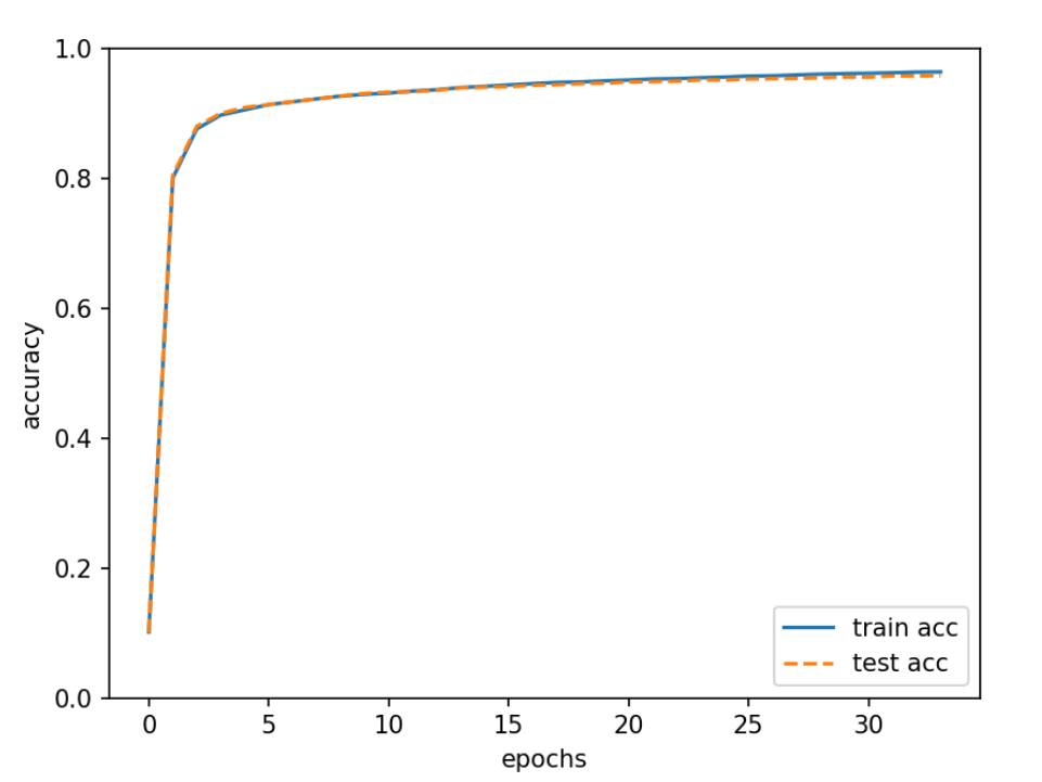
根据线状图可以看出我们的迭代次数越高，模型的准确率就越高。

另外本实验还利用了python当中的时间库求得了程序运行的总时间为：26.047357082366943秒。

7、实验心得

本次实验前，我对神经网络和反向传播算法的实现还不是很了解。然而，通过这个实验，我获得了宝贵的经验和知识。首先，我学习了神经网络的基本原理和结构。我了解到神经网络由输入层、隐藏层和输出层组成，每个层都包含多个神经元。这些神经元通过权重和偏置进行连接，并通过激活函数对输入进行转换其次，我深入学习了反向传播算法的原理。反向传播是一种训练神经网络的方法，它通过计算损失函数对权重和偏置进行调整，以使网络的输出尽可能接近期望的输出。这需要使用链式法则来计算每个神经元的梯度，并根据梯度下降算法来更新参数。我不仅学习了神经网络和反向传播算法的原理，还掌握了如何用C++实现一个简单的BP神经网络。这个实验让我对神经网络的工作原理有了更深入的理解，并为我今后的研究奠定了坚实的基础。