💥💥💞💞欢迎来到本博客❤️❤️💥💥

🏆博主优势：🌞🌞🌞博客内容尽量做到思维缜密，逻辑清晰，为了方便读者。

⛳️座右铭：行百里者，半于九十。

📋📋📋本文目录如下：🎁🎁🎁

目录

 ⛳️赠与读者

💥1 概述

📚2 运行结果

🎉3 参考文献

🌈4 Matlab代码、数据、文章下载

---

 ⛳️赠与读者

👨‍💻做科研，涉及到一个深在的思想系统，需要科研者逻辑缜密，踏实认真，但是不能只是努力，很多时候借力比努力更重要，然后还要有仰望星空的创新点和启发点。建议读者按目录次序逐一浏览，免得骤然跌入幽暗的迷宫找不到来时的路，它不足为你揭示全部问题的答案，但若能解答你胸中升起的一朵朵疑云，也未尝不会酿成晚霞斑斓的别一番景致，万一它给你带来了一场精神世界的苦雨，那就借机洗刷一下原来存放在那儿的“躺平”上的尘埃吧。

     或许，雨过云收，神驰的天地更清朗.......🔎🔎🔎

💥1 概述

摘要——本文提出了一种方法来实现四轴飞行器对目标的相对定位和跟踪使用超宽带（UWB）测距传感器，这些传感器被战略性地安装以帮助检索相对位置和四轴飞行器和目标之间的轴承。为了实现稳健即使在存在不确定性的情况下，也能实现自主飞行的本地化目标的速度，有两个主要特征。首先，开发了基于扩展卡尔曼滤波器（EKF）的估计器将超宽带测距测量结果与机载数据融合
传感器，包括惯性测量单元（IMU）、高度计以及光流。第二，要妥善处理目标方位与距离测量值，超宽带基于通信能力的通信能力被用来传输目标四轴飞行器的方向。实验结果表明四轴飞行器控制其相对于以下物体的位置的能力当目标静止时，在这两种情况下目标都是自主的和移动。超宽带鲁棒目标相对定位测距和通。

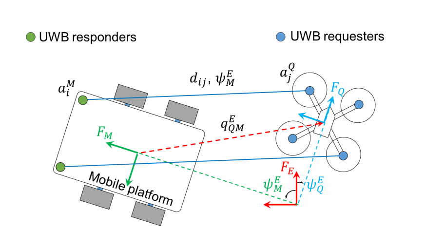
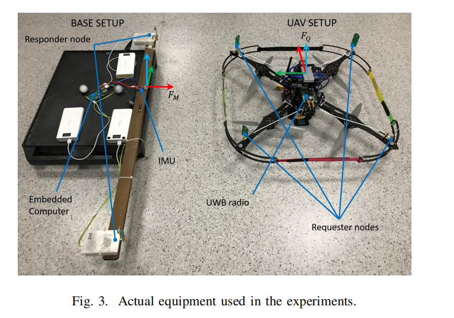
在多机器人系统中，通常期望每个机器人机器人能够确定其与其他机器人的相对位置执行诸如UGV-MAV（无人地面车辆-微型飞行器）车辆（微型飞行器）合作或移动形成。在这种和类似场景中，一种常见的方法是假设每个机器人都能确定自己的位置在一个全球共享的框架内，并将此信息传输给它的邻居。然而，基于卫星的系统，如GPS（全球定位系统）仅限于开放和整洁的户外环境。替代方法，如作为运动跟踪摄像机系统或基于无线电的定位系统，它们依赖于在以下区域进行仔细设置操作。后者的例子包括我们之前的工作基于超宽带定位[1]、[2]、[3]和类似的工作其他文献[4]、[5]。或者，一些作品假设具有某种接近感知能力。一种方法是使用距离传感方法例如红外距离传感器[6]或激光扫描仪7.然而，这种方法不能提供识别邻居之间相对而言范围较小。另一个高度一种有前景的方法，一直是热门的研究课题是使用计算机视觉系统。基于愿景该方法为所提出的系统提供了一个有利的替代方案本文虽有所论述，但并非没有局限性。参见[8]、[9]等，[10]. 简而言之，其局限性包括视野有限、时间短范围，以及可能要求计算能力，这是轻型空中机器人无法满足的。在本文中，我们提出了一种单目标相对定位系统单个移动机器人的定位。在这里，我们利用基于UWB的TWTOF（双向飞行时间）异步测距测量目标移动机器人，以确定相对位置，无需额外的外部设备。位置估计方法类似于我们的在文献[11]和[2]中，已经进行了先前的工作。代替放置多个锚点在作战区域，两台机器人都携带了多个UWB天线以适当的配置放置。此外，我们为MAV-UGV合作场景开发了该系统（图1），并将IMU、高度计和光学相关流量数据集成到扩展卡尔曼滤波器中，以提供足够准确和稳定的相对位置数据用于反馈控制飞行。这种基于测距的方法是全向的，并允许其他传感器（如摄像头）用于其他任务，而不是将其训练为目标[12]。使用该系统，MAV将能够在无人地面车辆周围进行精确定位，执行任务并与之精确对接。对于此类应用，UGV可以假设它们保持固定，但是在这项工作中，我们关注的是当目标为以下情况时，测试系统的鲁棒性移动，并且MAV不知道其速度。详细文章见第4部分。

📚2 运行结果

 

可视化部分代码：

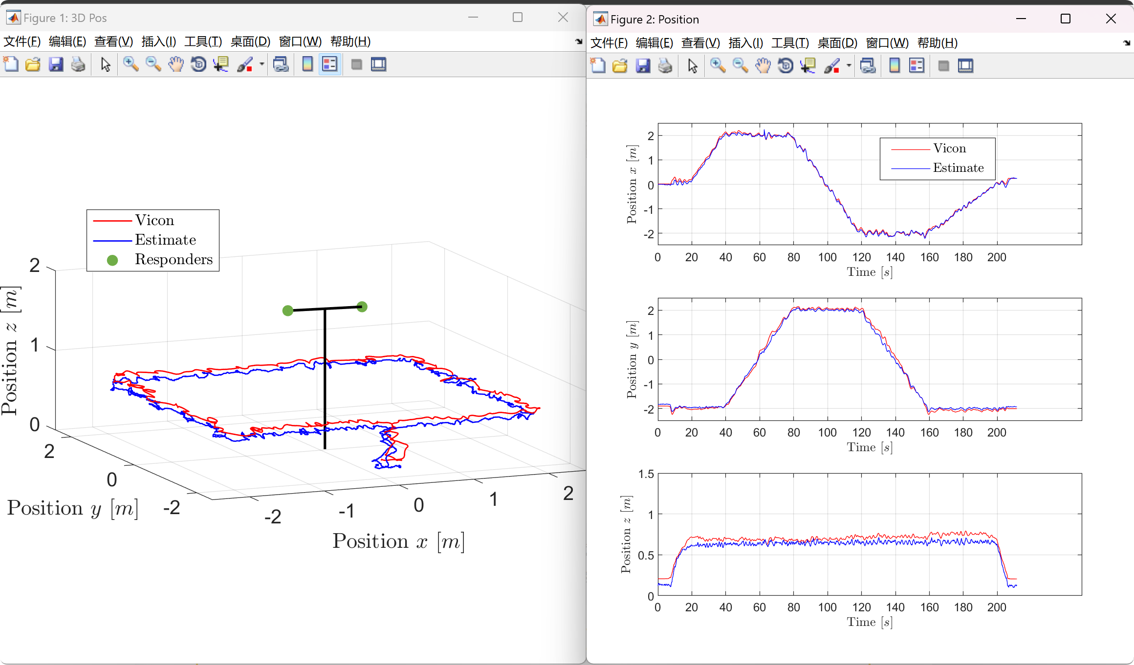
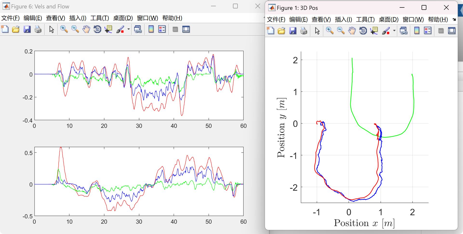
figure('name', '3D Pos', 'position', [865 200 400 400], 'color', [1 1 1]);
hold on;
vctarhd = plot3(vcTarP(1, :), vcTarP(2, :), vcTarP(3, :), 'g', 'linewidth', 1);
vcquadhd = plot3(vcP(1, :), vcP(2, :), vcP(3, :), 'r', 'linewidth', 1);
px4quadhd = plot3(px4P(1, :), px4P(2, :), px4P(3, :), 'b', 'linewidth', 1);
set(gca, 'DataAspectRatio', [1 1 1], 'fontsize', 14);
xlim([-1.5, 2.5]);
ylim([-2.5, 2.25]);
ylb = ylabel('$\mathrm{Position}\ y\ [m]$', 'interpreter', 'latex');%, 'position', [-9.2995 -14.2466 2.6102]);
xlabel('$\mathrm{Position}\ x\ [m]$', 'interpreter', 'latex');
zlabel('$\mathrm{Position}\ z\ [m]$', 'interpreter', 'latex');
grid on;

figure('name', 'Position','position', [1278 100 840 630], 'color', [1 1 1]);
subplot(3, 1, 1);
plot(t, vcP(1, :), 'r', t, px4P(1, :), 'b');
grid on;
set(gca, 'XTick',t(1):20:t(end));
xlabel('$\mathrm{Time}\ [s]$', 'interpreter', 'latex', 'fontsize', 14);
ylabel('$\mathrm{Position}\ x\ [m]$', 'interpreter', 'latex', 'fontsize', 14);
lghd = legend('$\mathrm{Vicon}$', '$\mathrm{Estimate}$');
set(lghd, 'interpreter', 'latex', 'fontsize', 14, 'position', [0.5360 0.8102 0.2117 0.1057]);
set(gca, 'fontsize', 16);  
grid on;

subplot(3, 1, 2);
plot(t, vcP(2, :), 'r', t, px4P(2, :), 'b');
grid on;
set(gca, 'XTick',t(1):20:t(end));
xlabel('$\mathrm{Time}\ [s]$', 'interpreter', 'latex', 'fontsize', 14);
ylabel('$\mathrm{Position}\ y\ [m]$', 'interpreter', 'latex', 'fontsize', 14);
set(gca, 'fontsize', 16);  

subplot(3, 1, 3);
plot(t, vcP(3, :), 'r', t, px4P(3, :), 'b');
grid on;
set(gca, 'XTick',t(1):20:t(end));
xlabel('$\mathrm{Time}\ [s]$', 'interpreter', 'latex', 'fontsize', 14);
ylabel('$\mathrm{Position}\ z\ [m]$', 'interpreter', 'latex', 'fontsize', 14);
set(gca, 'fontsize', 16);  

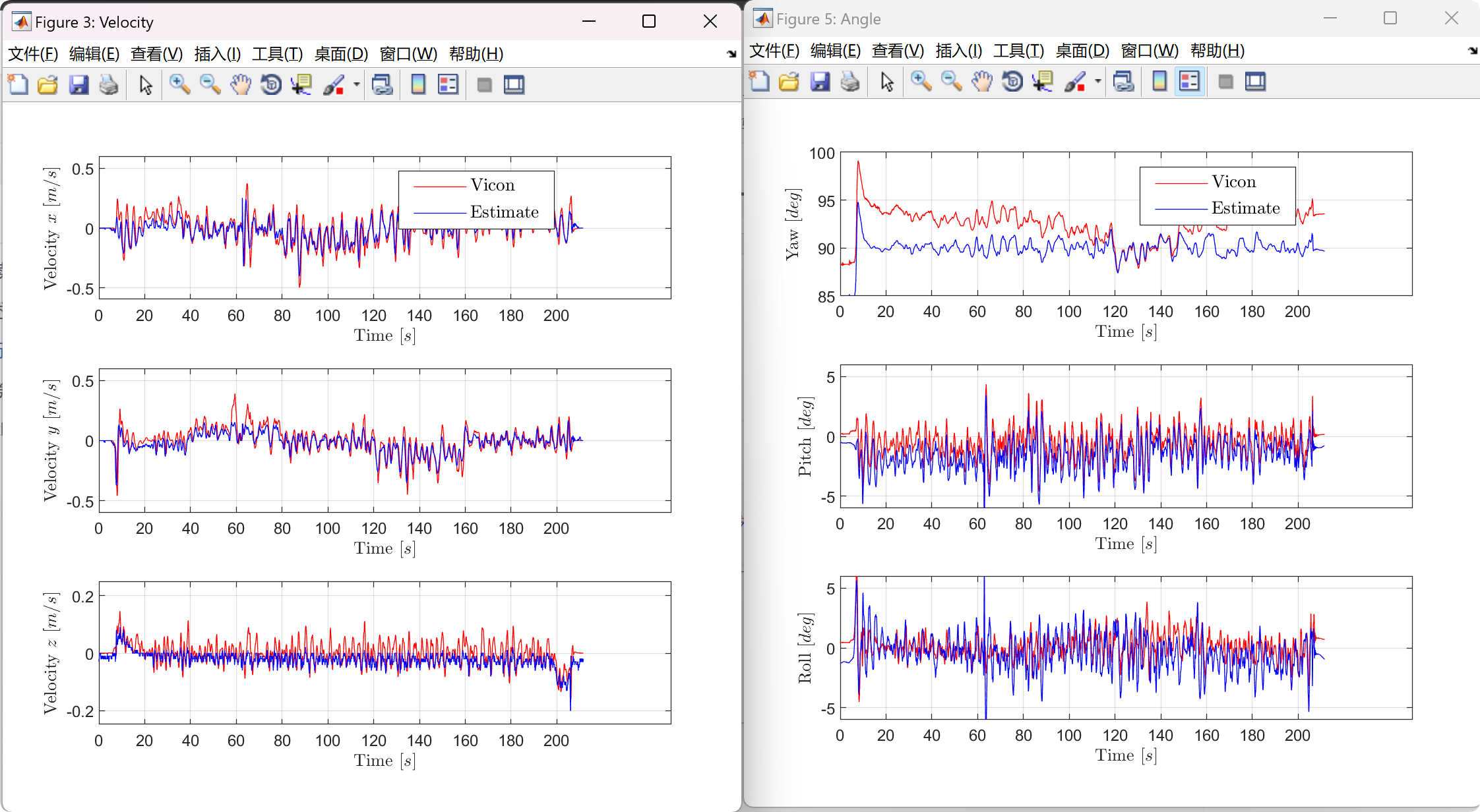
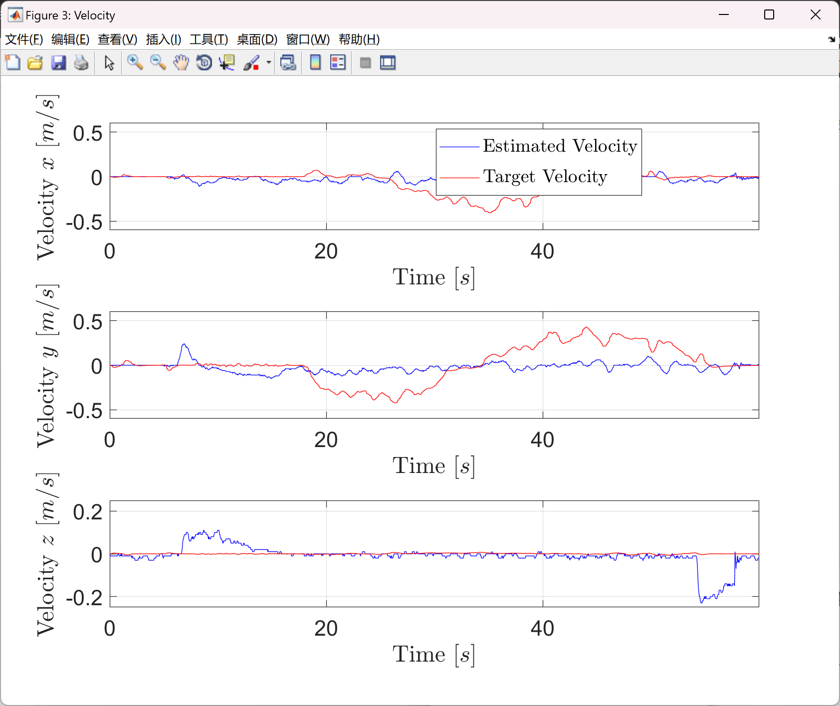
figure('name', 'Velocity','position', [1278 100 840 630], 'color', [1 1 1]);
subplot(3, 1, 1);
plot(t, px4V(1, :), 'b', t, vcTarV(1, :), 'r');
grid on;
ylim([-0.6, 0.6]);
set(gca, 'XTick',t(1):20:t(end));
xlabel('$\mathrm{Time}\ [s]$', 'interpreter', 'latex', 'fontsize', 14);
ylabel('$\mathrm{Velocity}\ x\ [m/s]$', 'interpreter', 'latex', 'fontsize', 14);
lghd = legend('$\mathrm{Estimated\ Velocity}$', '$\mathrm{Target\ Velocity}$');
set(lghd, 'interpreter', 'latex', 'fontsize', 14, 'position', [0.5360 0.8102 0.2117 0.1057]);
set(gca, 'fontsize', 16);  
grid on;

subplot(3, 1, 2);
plot(t, px4V(2, :), 'b', t, vcTarV(2, :), 'r');
grid on;
ylim([-0.6, 0.6]);
set(gca, 'XTick',t(1):20:t(end));
xlabel('$\mathrm{Time}\ [s]$', 'interpreter', 'latex', 'fontsize', 14);
ylabel('$\mathrm{Velocity}\ y\ [m/s]$', 'interpreter', 'latex', 'fontsize', 14);
set(gca, 'fontsize', 16);  

subplot(3, 1, 3);
plot(t, px4V(3, :), 'b', t, vcTarV(3, :), 'r');
grid on;
ylim([-0.25, 0.25]);
set(gca, 'XTick',t(1):20:t(end));
xlabel('$\mathrm{Time}\ [s]$', 'interpreter', 'latex', 'fontsize', 14);
ylabel('$\mathrm{Velocity}\ z\ [m/s]$', 'interpreter', 'latex', 'fontsize', 14);
set(gca, 'fontsize', 16);  

figure('name', 'Pos. Err', 'position', [2626 64 840 630], 'color', 'w');
plot(t, abs(vcP(1, :) - px4P(1, :)), 'r', t, abs(vcP(2, :) - px4P(2, :)), 'g', t, abs(vcP(3, :) - px4P(3, :)), 'b');
ylim([0, 0.2]);
xlabel('$\mathrm{Time}\ [s]$', 'interpreter', 'latex', 'fontsize', 14);
ylabel('$\mathrm{Error}\ x\ [m]$', 'interpreter', 'latex', 'fontsize', 14);
lghd = legend('$\mathrm{Position\ Error\ X}$', '$\mathrm{Position\ Error\ Y}$', '$\mathrm{Position\ Error\ Z}$');
set(lghd, 'interpreter', 'latex', 'fontsize', 14, 'position', [0.5360 0.8102 0.2117 0.1057]);
set(gca, 'fontsize', 16);  

rmsex = rms(vcP(1, :) - px4P(1, :));
rmsey = rms(vcP(2, :) - px4P(2, :));
rmsez = rms(vcP(3, :) - px4P(3, :));

stdx = std(vcP(1, :) - px4P(1, :));
stdy = std(vcP(2, :) - px4P(2, :));
stdz = std(vcP(3, :) - px4P(3, :));

rmsevx = rms(vcV(1, :) - px4V(1, :));
rmsevy = rms(vcV(2, :) - px4V(2, :));
rmsevz = rms(vcV(3, :) - px4V(3, :));

stdvx = std(vcV(1, :) - px4V(1, :));
stdvy = std(vcV(2, :) - px4V(2, :));
stdvz = std(vcV(3, :) - px4V(3, :));

maxTarVx = max(abs(vcTarV(1, :)));
maxTarVy = max(abs(vcTarV(2, :)));
maxTarVz = max(abs(vcTarV(3, :)));

uwbD = flightdata(:, end-3)';
ancAntId = floor(flightdata(:, end-2)'/16) + 1;
mobAntId = mod(flightdata(:, end-2)', 16) + 1;
rqstrId = flightdata(:, end)'-1;
rspdrId = flightdata(:, end-1)'+1;

[~, mobAnts] = size(mobAntOff);
[~, ancs] = size(ancPos);

edgeTotal = max(mobAnts*ancs);

f = [];

% uwbAllD = zeros(antCount, K);
vcD = zeros(1, K);
vcDCM = zeros(3, 3, K);
px4DCM = zeros(3, 3, K);

px4EulinVC = zeros(3, K);

vcMobAntPos = zeros(3, mobAnts*2, K);
vcAntPosCompact = zeros(3, K);

vcVbody = zeros(3, K);

for k = 1:K
    vcRo = vcEul(1, k);
    vcPi = vcEul(2, k);
    vcYa = vcEul(3, k);
    
    vcRx = [1, 0, 0; 0, cos(vcRo), -sin(vcRo); 0, sin(vcRo), cos(vcRo)];
    vcRy = [cos(vcPi), 0, sin(vcPi); 0, 1, 0; -sin(vcPi), 0, cos(vcPi)];
    vcRz = [cos(vcYa), -sin(vcYa), 0; sin(vcYa), cos(vcYa), 0; 0, 0, 1];
    
    vcDCM(:, :, k) = vcRx*vcRy*vcRz;
    
    px4Ro = px4Eul(1, k);
    px4Pi = px4Eul(2, k);
    px4Ya = px4Eul(3, k);
    
    px4Rx = [1, 0, 0; 0, cos(px4Ro), -sin(px4Ro); 0, sin(px4Ro), cos(px4Ro)];
    px4Ry = [cos(px4Pi), 1, sin(px4Pi); 0, 1, 0; -sin(px4Pi), 0, cos(px4Pi)];
    px4Rz = [cos(px4Ya), -sin(px4Ya), 0; sin(px4Ya), cos(px4Ya), 0; 0, 0, 1];
    
    px4DCM(:, :, k) = [0 1, 0; 1 0 0; 0 0 -1]*px4Rz*px4Ry*px4Rx*[1 0, 0; 0 -1 0; 0 0 -1];
    
    [px4Eul(1, k), px4Eul(2, k), px4Eul(3, k)] = dcm2angle(px4DCM(:, :, k)', 'XYZ');
    [vcEul(1, k), vcEul(2, k), vcEul(3, k)] = dcm2angle(vcDCM(:, :, k)', 'XYZ');
    
    for n=1:2
        for s=1:2
            vcMobAntPos(:, (n-1)*2 + s, k) = vcDCM(:, :, k)*mobAntOff(:, (n-1)*2 + s) + vcP(:, k);
        end
    end
    vcD(k) = norm(vcMobAntPos(:, (rqstrId(k)-1)*2 + mobAntId(k), k)...
                - (ancPos(:, rspdrId(k)) + ancAntOff(:, ancAntId(k))));
    vcAntPosCompact(:, k) = vcMobAntPos(:, (rqstrId(k)-1)*2 + mobAntId(k), k);
    
    vcVbody(:, k) = vcDCM(:, :, k)'*vcV(:, k);
    
    if flowpsr(k) > 40
        corflowvalid(:, k) = corflow(:, k);
    elseif k > 1
        corflowvalid(:, k) = corflowvalid(:, k-1);
    else
        corflowvalid(:, k) = [0; 0; 0];
    end
end

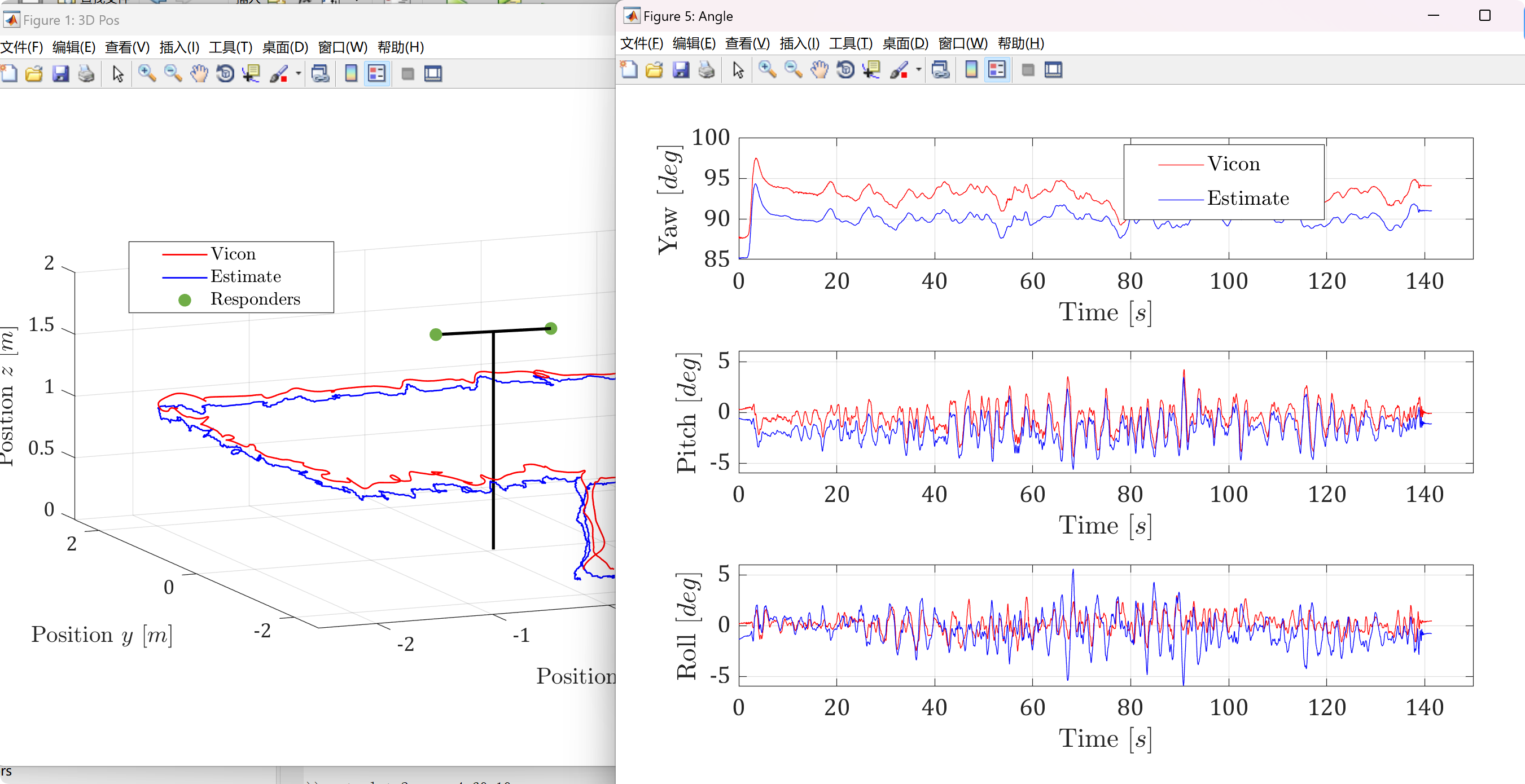
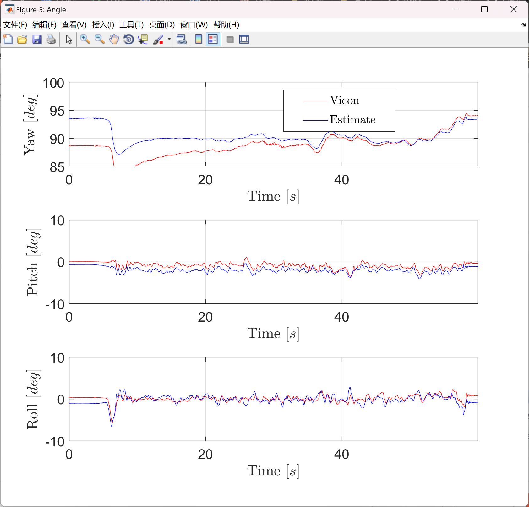
figure('name', 'Angle','position', [1278 100 840 630], 'color', [1 1 1]);
subplot(3, 1, 3);
plot(t, vcEul(1, :)*180/pi, 'r', t, px4Eul(1, :)*180/pi, 'b');
grid on;
ylim([-10, 10]);
set(gca, 'XTick',t(1):20:t(end));
xlabel('$\mathrm{Time}\ [s]$', 'interpreter', 'latex', 'fontsize', 14);
ylabel('$\mathrm{Roll}\ [deg]$', 'interpreter', 'latex', 'fontsize', 14);
set(gca, 'fontsize', 16);  

subplot(3, 1, 2);
plot(t, vcEul(2, :)*180/pi, 'r', t, px4Eul(2, :)*180/pi, 'b');
grid on;
ylim([-10, 10]);
set(gca, 'XTick',t(1):20:t(end));
xlabel('$\mathrm{Time}\ [s]$', 'interpreter', 'latex', 'fontsize', 14);
ylabel('$\mathrm{Pitch}\ [deg]$', 'interpreter', 'latex', 'fontsize', 14);
set(gca, 'fontsize', 16);  

subplot(3, 1, 1);
% plot(t, vcP(3, :), 'r', t, px4P(3, :), 'b', t, px4Lidar, 'g');
plot(t, vcEul(3, :)*180/pi, 'r', t, px4Eul(3, :)*180/pi, 'b');
grid on;
ylim([85, 100]);
set(gca, 'XTick',t(1):20:t(end));
xlabel('$\mathrm{Time}\ [s]$', 'interpreter', 'latex', 'fontsize', 14);
ylabel('$\mathrm{Yaw}\ [deg]$', 'interpreter', 'latex', 'fontsize', 14);
lghd = legend('$\mathrm{Vicon}$', '$\mathrm{Estimate}$');
set(lghd, 'interpreter', 'latex', 'fontsize', 14, 'position', [0.5360 0.8102 0.2117 0.1057]);
set(gca, 'fontsize', 16);  

rmseyaw = rms(vcEul(3, :)*180/pi - px4Eul(3, :)*180/pi);
rmsepitch = rms(vcEul(2, :)*180/pi - px4Eul(2, :)*180/pi);
rmseroll = rms(vcEul(1, :)*180/pi - px4Eul(1, :)*180/pi);

stdyaw = std(vcEul(3, :)*180/pi - px4Eul(3, :)*180/pi);
stdpitch = std(vcEul(2, :)*180/pi - px4Eul(2, :)*180/pi);
stdroll = std(vcEul(1, :)*180/pi - px4Eul(1, :)*180/pi);

errsig = round([rmsex, rmsey, rmsez, maxTarVx, maxTarVy, maxTarVz;
                stdx, stdy, stdz, 0, 0, 0], 3);

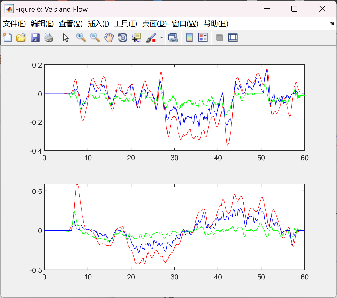
figure('name', 'Vels and Flow', 'position', [865 100 560 420]);
subplot(2, 1, 1);
plot(t, vcV(1, :), 'r', t, px4V(1, :), 'g', t, corflow(1, :).*vcP(3, :), 'b');
subplot(2, 1, 2);
plot(t, vcV(2, :), 'r', t, px4V(2, :), 'g', t, -corflow(2, :).*vcP(3, :), 'b');

🎉3 参考文献

文章中一些内容引自网络，会注明出处或引用为参考文献，难免有未尽之处，如有不妥，请随时联系删除。(文章内容仅供参考，具体效果以运行结果为准)

🌈4 Matlab代码、数据、文章下载

资料获取，更多粉丝福利，MATLAB|Simulink|Python资源获取