神经网络-损失函数-等高线理解

经常会有人用等高线理解一些事情，那么什么是等高线能用程序画出下面这个函数的损失函数的等高线K是神经网络一个神经元的权重Wb是一个神经元的偏移值Y=kx+b图片import mathimport randomimport numpy as npimport matplotlib.pyplot as pltx_train = np.array([0,1,2,3...

茫茫人海一粒沙

6042人浏览 · 2020-04-19 20:01:29

茫茫人海一粒沙 · 2020-04-19 20:01:29 发布

一，等高线理解

如果一个变量 w
$=\frac{1}{m}\sum_i(wx_i -y_i)^2$

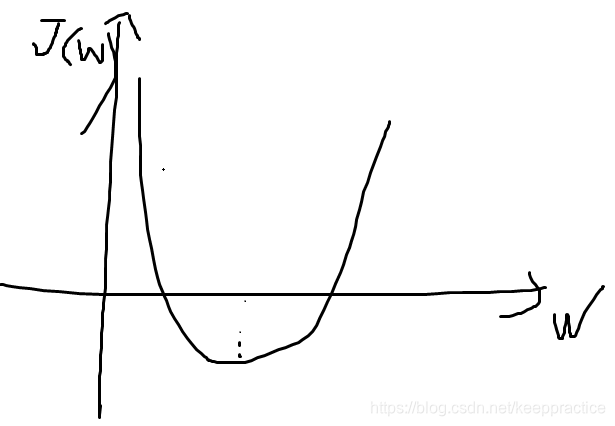
2/ 如果有两个变量 w与b
$=\frac{1}{m}\sum_i(wx_i+b -y_i)^2$
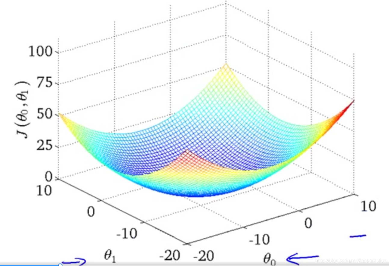
等高线就是把上面这个三维图片映射到二维平面上

二，用程序画出下面这个函数的损失函数的等高线

K是神经网络一个神经元的权重W
b是一个神经元的偏移值

Y=kx+b

y 期望值
损失函数
$=\frac{1}{m} (Y - y)^2$

图片
在这里插入图片描述

import math
import random
import numpy as np
import matplotlib.pyplot as plt

x_train = np.array([0,   1,	  2,   3,   4,   5])
y_train = np.array([1.1, 2.2,  3.8, 4.1, 4.9, 5.2])

dense = 200
k = np.linspace(0,2,dense)
b = np.linspace(-2,4,dense)

# y = kx+b
def get_loss_value(k,b):
    return np.square(k*x_train+b - y_train).sum()/len(x_train)

def draw_contour_line(dense,isoheight): #dense表示取值的密度，isoheight表示等高线的值
    list_k = []
    list_b = []
    list_loss = []
    for i in range(dense):
        for j in range(dense):
            loss = get_loss_value(k[i],b[j])
            if 1.05*isoheight>loss>0.95*isoheight:
                list_k.append(k[i])
                list_b.append(b[j])
            else:
                pass
    plt.scatter(list_k,list_b,s=1) #s=0.25比较合适

draw_contour_line(dense,0.2)
draw_contour_line(dense,0.5)
draw_contour_line(dense,0.7)
draw_contour_line(dense,1)
draw_contour_line(dense,3)
draw_contour_line(dense,8)
draw_contour_line(dense,10)
draw_contour_line(dense,15)
draw_contour_line(dense,20)
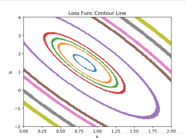
plt.title('Loss Func Contour Line')
plt.xlabel('k')
plt.ylabel('b')
plt.axis([0,2,-2,4])
plt.show()

图1是没有标准化输入X的等高线图
图2是标准化输入X的等高线图
可以看到标准化等高线图像是放正了的椭圆
Y=kx+b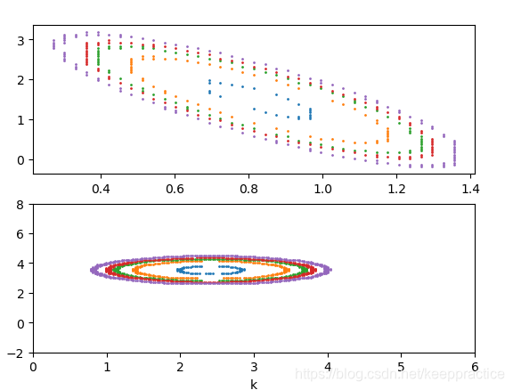
在这里插入图片描述

import math
import random
import numpy as np
import matplotlib.pyplot as plt

def tanh(x):
    return (np.exp(x)-np.exp(-x))/(np.exp(x)+np.exp(-x))

def sigmoid(x):
    return 1/(1+np.exp(-x))

def relu(x):
	return np.maximum(x, 0)

def transfor_stardard(x):
    x_mean = np.mean(x)
    x_var = np.var(x, axis=0)
    return (x - x_mean) / x_var

x_train = np.array([0,   1,	  2,   3,   4,   5])
y_train = np.array([1.1, 2.2,  3.8, 4.1, 4.9, 5.2])

x_train_stardard = transfor_stardard(x_train)
print(x_train_stardard)

dense = 200
k = np.linspace(0,6,dense)
b = np.linspace(-2,8,dense)


def activate(x):
    #return tanh(x)
    #return transfor_stardard(sigmoid(x))
    return x


# y = kx+b
def get_loss_value(k,b):
    return np.square(activate(k*x_train+b - y_train)).sum()/len(x_train)
def get_loss_value_with_stardard(k,b):
    return np.square(activate(k*x_train_stardard+b - y_train)).sum()/len(x_train)

def draw_contour_line(dense,isoheight): #dense表示取值的密度，isoheight表示等高线的值
    list_k = []
    list_b = []

    list_loss = []
    for i in range(dense):
        for j in range(dense):
            loss = get_loss_value(k[i],b[j])
            if 1.05*isoheight>loss>0.95*isoheight:
                list_k.append(k[i])
                list_b.append(b[j])
            else:
                pass
    plt.subplot(211)
    plt.scatter(list_k, list_b, s=1)  # s=0.25比较合适
    list_k_stardard = []
    list_b_stardard = []
    for i in range(dense):
        for j in range(dense):
            loss_stardard = get_loss_value_with_stardard(k[i], b[j])
            if 1.05 * isoheight > loss_stardard > 0.95 * isoheight:
                list_k_stardard.append(k[i])
                list_b_stardard.append(b[j])
            else:
                pass
    plt.subplot(212)
    plt.scatter(list_k_stardard, list_b_stardard, s=1)  # s=0.25比较合适


draw_contour_line(dense,0.2)
draw_contour_line(dense,0.5)
draw_contour_line(dense,0.7)
draw_contour_line(dense,0.8)
draw_contour_line(dense,1)
#plt.title('Loss Func Contour Line')
plt.xlabel('k')
plt.ylabel('b')
plt.axis([0,6,-2,8])
plt.show()

损失函数
$=\frac{1}{m} (Y - y)^2$
且Y=kx+b 的3D 图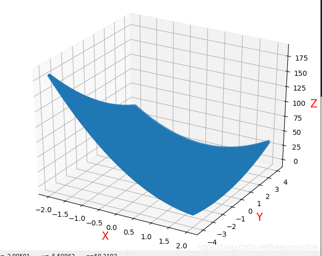
在这里插入图片描述
损失函数
$=\frac{1}{m} (Y - y)^2$
且Y=tanh(kx+b) 的3D 图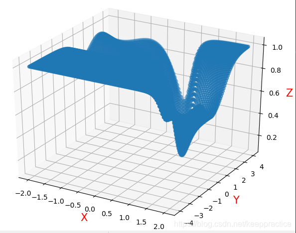

import math
import random
import numpy as np
import matplotlib.pyplot as plt

from mpl_toolkits.mplot3d import Axes3D
def tanh(x):
    return (np.exp(x)-np.exp(-x))/(np.exp(x)+np.exp(-x))

x_train = np.array([0, 1, 2, 3, 4, 5])
y_train = np.array([1.1, 2.2, 3.8, 4.1, 4.9, 5.2])

dense = 100
k = np.linspace(-2, 2, dense)
b = np.linspace(-4, 4, dense)
def get_loss_value(k, b):
    return np.square(k * x_train + b - y_train).sum() / len(x_train)
def draw_3D_diagram(dense):  # dense表示取值的密度，isoheight表示等高线的值
    list_k = []
    list_b = []
    list_loss = []
    for i in range(dense):
        for j in range(dense):
            list_k.append(k[i])
            list_b.append(b[j])
            loss = get_loss_value(k[i], b[j])
            list_loss.append(loss)
    fig = plt.figure()
    ax = Axes3D(fig)
    ax.scatter(list_k, list_b, list_loss)
    # xmin xmax ymin ymax
    ax.set_zlabel('Z', fontdict={'size': 15, 'color': 'red'})
    ax.set_ylabel('Y', fontdict={'size': 15, 'color': 'red'})
    ax.set_xlabel('X', fontdict={'size': 15, 'color': 'red'})

draw_3D_diagram(dense)

plt.show()

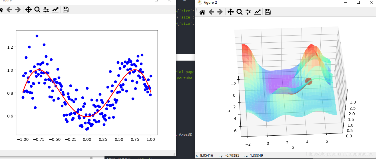
用 Tensorflow 可视化梯度下降

在这里插入图片描述


import tensorflow as tf
import numpy as np
import matplotlib.pyplot as plt
from mpl_toolkits.mplot3d import Axes3D

LR = 0.1
REAL_PARAMS = [1.2, 2.5]
INIT_PARAMS = [[5, 4],
               [5, 1],
               [2, 4.5]][2]

x = np.linspace(-1, 1, 200, dtype=np.float32)   # x data

# Test (1): Visualize a simple linear function with two parameters,
# you can change LR to 1 to see the different pattern in gradient descent.

# y_fun = lambda a, b: a * x + b
# tf_y_fun = lambda a, b: a * x + b


# Test (2): Using Tensorflow as a calibrating tool for empirical formula like following.

# y_fun = lambda a, b: a * x**3 + b * x**2
# tf_y_fun = lambda a, b: a * x**3 + b * x**2


# Test (3): Most simplest two parameters and two layers Neural Net, and their local & global minimum,
# you can try different INIT_PARAMS set to visualize the gradient descent.

y_fun = lambda a, b: np.sin(b*np.cos(a*x))
tf_y_fun = lambda a, b: tf.sin(b*tf.cos(a*x))

noise = np.random.randn(200)/10
y = y_fun(*REAL_PARAMS) + noise         # target

# tensorflow graph
a, b = [tf.Variable(initial_value=p, dtype=tf.float32) for p in INIT_PARAMS]
pred = tf_y_fun(a, b)
mse = tf.reduce_mean(tf.square(y-pred))
train_op = tf.train.GradientDescentOptimizer(LR).minimize(mse)

a_list, b_list, cost_list = [], [], []
with tf.Session() as sess:
    sess.run(tf.global_variables_initializer())
    for t in range(400):
        a_, b_, mse_ = sess.run([a, b, mse])
        a_list.append(a_); b_list.append(b_); cost_list.append(mse_)    # record parameter changes
        result, _ = sess.run([pred, train_op])                          # training


# visualization codes:
print('a=', a_, 'b=', b_)
plt.figure(1)
plt.scatter(x, y, c='b')    # plot data
plt.plot(x, result, 'r-', lw=2)   # plot line fitting
# 3D cost figure
fig = plt.figure(2); ax = Axes3D(fig)
a3D, b3D = np.meshgrid(np.linspace(-2, 7, 30), np.linspace(-2, 7, 30))  # parameter space
cost3D = np.array([np.mean(np.square(y_fun(a_, b_) - y)) for a_, b_ in zip(a3D.flatten(), b3D.flatten())]).reshape(a3D.shape)
ax.plot_surface(a3D, b3D, cost3D, rstride=1, cstride=1, cmap=plt.get_cmap('rainbow'), alpha=0.5)
ax.scatter(a_list[0], b_list[0], zs=cost_list[0], s=300, c='r')  # initial parameter place
ax.set_xlabel('a'); ax.set_ylabel('b')
ax.plot(a_list, b_list, zs=cost_list, zdir='z', c='r', lw=3)    # plot 3D gradient descent
plt.show()

参考资料
[1] https://blog.csdn.net/bitcarmanlee/article/details/85275016

技术共进，成长同行——讯飞AI开发者社区

更多推荐

AI智能体—人工智能工作流与人工智能智能体：真正的区别是什么？

本文探讨了人工智能工作流与智能体的核心区别。工作流是静态、可预测的执行序列（如预处理→嵌入→搜索→总结），适合批处理作业；而智能体能动态感知环境、自主决策（感知→推理→决策循环），具备适应性和工具选择能力。关键差异在于：工作流遵循固定路径，智能体则能根据目标调整策略。架构上，工作流使用Airflow等工具，智能体依赖LangChain等框架。智能体的自主性使其更适用于动态环境，代表下一代AI应用方