目录

一、理论基础

1.1、MNIST手写数字数据库

1.2、CNN深度学习网络

1.3、MNIST手写数字识别实现

1.4、总结

二、核心程序

三、仿真结论

---

一、理论基础

       手写数字识别是机器学习领域中的一个重要应用，它可以应用于自动化数据输入、智能检测等领域。MNIST手写数字数据库是机器学习领域中的一个经典数据集，包含了一系列手写数字图片和对应的标签，是进行手写数字识别算法研究和性能评估的标准数据集之一。本文将介绍基于CNN深度学习网络的MNIST手写数字数据库训练和识别的实现方法和步骤。

1.1、MNIST手写数字数据库

      MNIST手写数字数据库是一个常用的手写数字识别数据集，包含了60000个训练集和10000个测试集。每个样本都是28x28像素的灰度图像，表示了0~9之间的数字。其中，训练集用于训练模型，测试集用于测试模型的准确率。

1. 标签信息： 标签是用于标识图像中手写数字的数字，范围从0到9。例如，标签0表示图像中的手写数字是数字0，标签1表示数字1，以此类推。

2. 数据的应用： MNIST数据集常被用作数字识别问题的基准数据集，尤其是在机器学习领域。研究者和开发者可以使用MNIST数据集来验证算法、模型或方法的性能。例如，可以将MNIST数据集用于训练和测试各种图像分类算法，如卷积神经网络（CNN）、支持向量机（SVM）等。

3. 数据获取： MNIST数据集可以从官方网站或许多开源机器学习库中获取，如TensorFlow、PyTorch等。这些库提供了方便的函数和接口，可以轻松加载和处理MNIST数据集。

4. 数据预处理： 在使用MNIST数据集之前，通常需要进行一些数据预处理，以适应具体的任务和模型。预处理可能包括图像归一化（将像素值缩放到0到1之间）、数据增强（生成变换后的图像以增加样本数量）等。

5. 应用领域： MNIST数据集的主要应用领域包括数字识别、图像分类、模式识别等。它被用于教育、学术研究以及算法验证和性能评估。

       MNIST手写数字数据库作为一个经典的数据集，为机器学习领域提供了一个常用的基准，有助于研究人员和开发者更好地理解和实验数字识别算法。同时，它也促进了新算法和模型的发展，为图像处理和模式识别领域做出了重要贡献。

1.2、CNN深度学习网络

       CNN（Convolutional Neural Network，卷积神经网络）是一种深度学习网络，特别适用于图像分类和识别任务。与传统神经网络不同，CNN可以自动提取数据的特征，从而实现对图像的高效分类和识别。CNN网络的核心组件包括卷积层、池化层和全连接层。

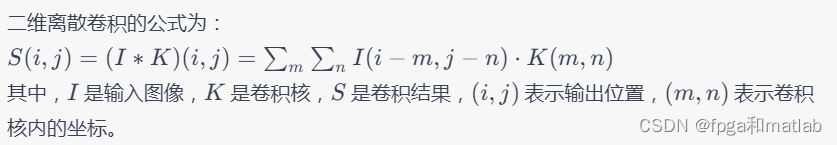
卷积层
       卷积层是CNN网络中的核心组件，它可以自动提取输入图像的特征。在卷积层中，使用一组可学习的卷积核对输入图像进行卷积操作，得到一组特征图。卷积核是一个小的矩阵，可以通过反向传播算法进行训练，以提取输入图像的不同特征。

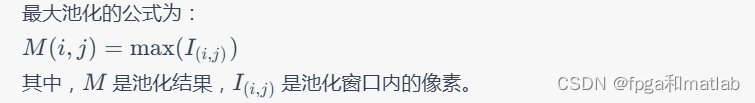
 池化层
      池化层是CNN网络中的另一个核心组件，它用于对特征图进行降维操作。在池化层中，通常使用最大池化或平均池化等操作，将每个特征图中的一定区域进行压缩，从而减少网络中的参数数量和计算量。

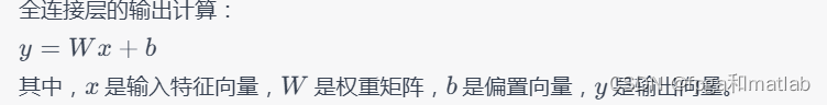
 全连接层
      全连接层是CNN网络中的最后一层，它用于对特征图进行分类。在全连接层中，可以使用softmax函数将特征图映射到0~1之间的概率值，从而得到对输入图像的分类结果。

1.3、MNIST手写数字识别实现

       基于CNN深度学习网络的MNIST手写数字识别实现主要包括以下几个步骤：数据集加载、数据预处理、模型构建、模型训练和模型测试。下面将逐一介绍这些步骤的具体实现方法。这个模型包含了两个卷积层、两个池化层和两个全连接层。在卷积层和全连接层中，都使用了ReLU激活函数来增强模型的非线性表达能力。在最后的全连接层中，使用了softmax函数来将特征图映射为概率值。

1.4、总结

       本文介绍了基于CNN深度学习网络的MNIST手写数字识别实现方法和步骤。通过对数据集的加载、预处理、模型构建、模型训练和模型测试等步骤的介绍，可以帮助读者了解深度学习网络的基本原理和实现方法，以及如何应用深度学习网络进行手写数字识别任务。
 

二、核心程序

clc;
clear;
close all;
warning off;
addpath(genpath(pwd));
rng('default')


inputSize  = 28 * 28;
numLabels  = 5;
hiddenSize = 200;
sparsityParam = 0.1; % desired average activation of the hidden units.
                     % (This was denoted by the Greek alphabet rho, which looks like a lower-case "p",
		             %  in the lecture notes). 
lambda = 3e-3;       % weight decay parameter       
beta = 3;            % weight of sparsity penalty term   

%% ======================================================================
%  STEP 1: Load data from the MNIST database
 

% Load MNIST database files
mnistData   = loadMNISTImages('mnist/train-images-idx3-ubyte');
mnistLabels = loadMNISTLabels('mnist/train-labels-idx1-ubyte');

% Set Unlabeled Set (All Images)

% Simulate a Labeled and Unlabeled set
labeledSet   = find(mnistLabels >= 0 & mnistLabels <= 4);
unlabeledSet = find(mnistLabels >= 5);

numTrain = round(numel(labeledSet)/2);
trainSet = labeledSet(1:numTrain);
testSet  = labeledSet(numTrain+1:end);

unlabeledData = mnistData(:, unlabeledSet);

trainData   = mnistData(:, trainSet);
trainLabels = mnistLabels(trainSet)' + 1; % Shift Labels to the Range 1-5

testData   = mnistData(:, testSet);
testLabels = mnistLabels(testSet)' + 1;   % Shift Labels to the Range 1-5

% Output Some Statistics
fprintf('# examples in unlabeled set: %d\n', size(unlabeledData, 2));
fprintf('# examples in supervised training set: %d\n\n', size(trainData, 2));
fprintf('# examples in supervised testing set: %d\n\n', size(testData, 2));

%% ======================================================================
%  STEP 2: Train the sparse autoencoder
 
theta = initializeParameters(hiddenSize, inputSize);

 
addpath minFunc/
autoencoderOptions.Method = 'lbfgs';  % Here, we use L-BFGS to optimize our cost
                                      % function. Generally, for minFunc to work, you
                                      % need a function pointer with two outputs: the
                                      % function value and the gradient. In our problem,
                                      % sparseAutoencoderCost.m satisfies this.
autoencoderOptions.maxIter = 400;	  % Maximum number of iterations of L-BFGS to run 
autoencoderOptions.display = 'on';

if exist('opttheta.mat','file')==2
    
    load('opttheta.mat');

else
[opttheta, cost] = minFunc( @(p) sparseAutoencoderCost(p, ...
                                   inputSize, hiddenSize, ...
                                   lambda, sparsityParam, ...
                                   beta, unlabeledData), ...
                              theta, autoencoderOptions);                        
save('opttheta.mat','opttheta');
end


%% -----------------------------------------------------
                          
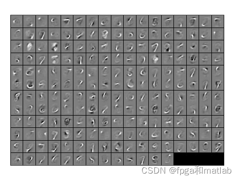
% Visualize weights
W1 = reshape(opttheta(1:hiddenSize * inputSize), hiddenSize, inputSize);
display_network(W1');

%%======================================================================
%% STEP 3: Extract Features from the Supervised Dataset
 

trainFeatures = feedForwardAutoencoder(opttheta, hiddenSize, inputSize, ...
                                       trainData);

testFeatures = feedForwardAutoencoder(opttheta, hiddenSize, inputSize, ...
                                       testData);

%%======================================================================
%% STEP 4: Train the softmax classifier
 

softmaxOptions.maxIter = 100;
lambdaSoftmax = 1e-4; % Weight decay parameter for Softmax
trainNumber = size(trainData,2);

% softmaxTrain 默认数据中已包含截距项
softmaxModel = softmaxTrain(hiddenSize+1, numLabels, lambdaSoftmax, [trainFeatures;ones(1,trainNumber)], trainLabels, softmaxOptions);  % learn by features
%softmaxModel = softmaxTrain(inputSize+1, numLabels, lambdaSoftmax, [trainData;ones(1,trainNumber)], trainLabels, softmaxOptions);  % learn by raw data


%% -----------------------------------------------------


%%======================================================================
%% STEP 5: Testing 

%% ----------------- YOUR CODE HERE ----------------------
% Compute Predictions on the test set (testFeatures) using softmaxPredict
% and softmaxModel
testNumber = size(testData,2);

% softmaxPredict 默认数据中已包含截距项
[pred] = softmaxPredict(softmaxModel, [testFeatures;ones(1,testNumber)]);  % predict by test features
%[pred] = softmaxPredict(softmaxModel, [testData;ones(1,testNumber)]);  % predict by test raw data


%% -----------------------------------------------------

% Classification Score
fprintf('Test Accuracy: %f%%\n', 100*mean(pred(:) == testLabels(:)));
up2112

三、仿真结论