目录

1.算法原理简介

2. 算法流程¶

3. 第一个例子，基于sklearn生成数据集

3.1 生成数据

 3.2 构建模型、训练及预测

4. 第二个例子，基于breast_cancer数据集¶

5. 决策边界与模型复杂度

6. 优缺点

---

1.算法原理简介

        kNN(k-Nearest Neighbors)算法，即k近邻算法可以说是最简单的机器学习算法，简单到kNN算法模型的构建都不需要训练，收集有标签数据样本就完事了！

        kNN算法的核心思想是：未知样本对应的target值由“距离”其最近的“k”个样本按照既定的“决策机制”进行决定。正所谓：近朱者赤近墨者黑。

        在以上核心思想描述中，三个由双引号圈起的概念恰好就构成kNN算法的三个基本要素：

        (1) 距离度量，或者说相似度。其中最常用的自然是欧几里得度量(euclidean metric)(也称欧氏距离)，本文仅考虑欧氏距离。考虑N维向量空间𝑅𝑁RN中的两个向量𝐱x和𝐲y，它们的欧氏距离定义为：

                

                

        除了欧氏距离外，机器学习中常用的距离(相似性)度量还有，曼哈顿距离(Manhattan distance)，切比雪夫距离(Chebyshev distance)，闵可夫斯基距离(Minkowski distance)，汉明距离(Hamming distance)，余弦相似度(Cosine Similarity),等等。需要根据实际问题的类型选择合适的距离度量，当然合适的距离度量选择是机器学习中的一个普遍问题，而不仅限于kNN。

        (2) 参数k。参数k反映了模型的复杂度。小的k值表示更复杂的模型；大的k值对应更简单的模型。k值的选择反映了对近似误差与估计误差之间的权衡，通常通过交叉验证搜索最优值。

        (3) 决策机制，即k个近邻基于什么样的机制来决定当前样本的值。通常最常用的就是多数表决(majority voting)，通俗地说就是少数服从多数。多数表决机制，对应于经验风险最小化（与之对应的有结构风险最小化）。

        k近邻模型对应于基于训练数据集对特征空间的一个划分。近邻法中，当训练集、距离度量、值及分类决策规则确定后，其结果唯一确定。

        kNN算法既可以用于回归问题（target值就是样本对应的预测值），也可以用于分类问题（target值就是样本的分类），不过一般情况下用于分类问题更加常见。本文以下也只考虑采用多数表决机制的kNN分类问题。

2. 算法流程¶

        记训练数据样本集为，包含N个样本。待预测样本为。kNN算法的基本算法流程如下：

        1.计算待预测数据样本与训练集中各样本数据之间的距离:

                

        2.按照距离的递增关系进行排序，并取距离最小的k个样本，记为

        3.统计中各类别出现的次数 

        4.取中出现次数最多的类别作为的预测分类

3. 第一个例子，基于sklearn生成数据集

        以下首先基于sklearn提供的make_blobs()函数生成一个玩具数据集(Ref: 机器学习笔记：常用数据集之scikit-learn生成分类和聚类数据集_chenxy_bwave的专栏-CSDN博客)

3.1 生成数据

# make_blobs: Generate isotropic Gaussian blobs for clustering. Of course, can also be used for classfication problem.
import pandas as pd
import numpy as np
import matplotlib.pyplot as plt
 
from sklearn.datasets import make_blobs

centers = [[-3, 3], [3, 3], [0, 6]]

X, y = make_blobs(n_samples=150, centers=centers, n_features=2,random_state=10, cluster_std=0.8)
 
# scatter plot, dots colored by class value
df = pd.DataFrame(dict(x=X[:,0], y=X[:,1], label=y))
colors = {0:'red', 1:'blue',2:'y'}
fig, ax = plt.subplots(figsize=(12,8))
grouped = df.groupby('label')
for key, group in grouped:
    group.plot(ax=ax, kind='scatter', s=80, x='x', y='y', label=key, color=colors[key])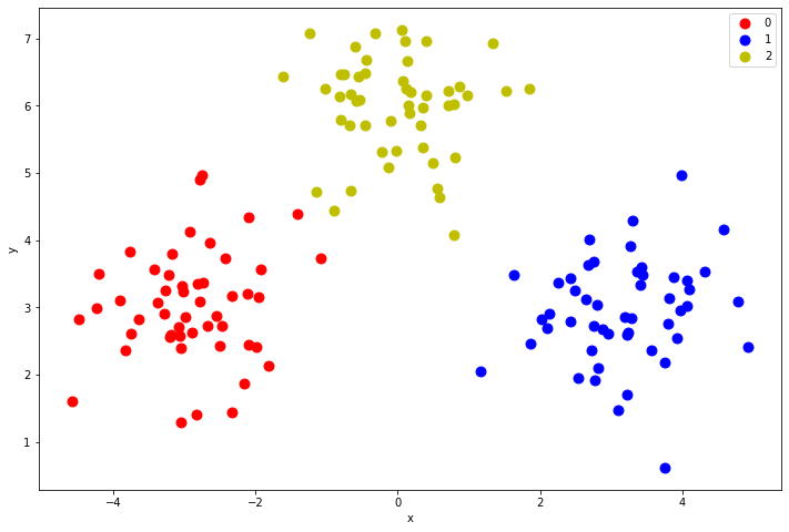

 3.2 构建模型、训练及预测

from sklearn.neighbors import KNeighborsClassifier
# 构建模型训练
k = 5
clf = KNeighborsClassifier(n_neighbors=k)
clf.fit(X, y);

# 进行预测
X_sample = np.array([[0, 2]]) # clf.predict expect 2-D array as input.
y_sample = clf.predict(X_sample);
neighbors = clf.kneighbors(X_sample, return_distance=False); 
    # returns 2-D array, including the indexes of k-neighbor samples in the original dataset
    
print('{0} is predicted to belong to class#{1}'.format(X_sample,y_sample))    
print('and, its nearear neighbors are: ', neighbors)

[[0 2]] is predicted to belong to class#[0]
and, its nearear neighbors are:  [[ 15  54  78 121  93]]

        注意，虽然调用了fit()函数，但是如前所述，KNN的fit()函数并没有做啥，只是记录训练数据集而已。以上样本预测例图示如下：

# 画出示意图
cts = np.array(centers)
plt.figure(figsize=(10, 8), dpi=100)
plt.scatter(X[:, 0], X[:, 1], c=y, s=80, cmap='cool');    # 样本
plt.scatter(cts[:, 0], cts[:, 1], s=80, marker='^', c='k');   # 中心点
plt.scatter(X_sample[:,0], X_sample[:,1], marker="x", 
            c=y_sample, s=80, cmap='cool')    # 待预测的点

for i in neighbors[0]:
    plt.plot([X[i][0], X_sample[0][0]], [X[i][1], X_sample[0][1]], 
             'k--', linewidth=0.6);    # 预测点与距离最近的k个样本的连线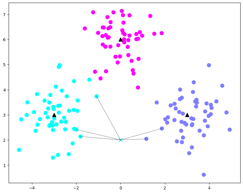

 

4. 第二个例子，基于breast_cancer数据集¶

        Ref: Introduction to Machine Learning with Python, by Andreas C.Muller

        在以下模型中，对比了k从1到10变化对于模型的性能的影响。这里考察的性能度量为预测准确度(accuracy)，在scikit-learn中可以调用分类器对象的score()方法给出。以下同时给出在训练集和测试集上的accuracy随着参数k的变化为变化的情况。

from sklearn.datasets import load_breast_cancer
from sklearn.model_selection import train_test_split

cancer = load_breast_cancer()
X_train, X_test, y_train, y_test = train_test_split(
    cancer.data, cancer.target, stratify=cancer.target, random_state=66)

training_accuracy = []
test_accuracy = []
# try n_neighbors from 1 to 10
neighbors_settings = range(1, 11)

for n_neighbors in neighbors_settings:
    # build the model
    clf = KNeighborsClassifier(n_neighbors=n_neighbors)
    clf.fit(X_train, y_train)
    # record training set accuracy
    training_accuracy.append(clf.score(X_train, y_train))
    # record generalization accuracy
    test_accuracy.append(clf.score(X_test, y_test))
    
plt.plot(neighbors_settings, training_accuracy, label="training accuracy")
plt.plot(neighbors_settings, test_accuracy, label="test accuracy")
plt.ylabel("Accuracy")
plt.xlabel("n_neighbors")
plt.legend()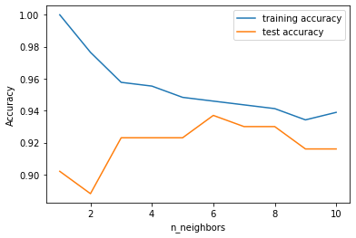

 

        由上图可以看出，随着k的增大，在训练集上的预测准确度逐渐下降，而测试集上的预测准确度开始阶段是增大，但是到了一定阶段后就又开始下降。

        尤其是，当k=1时，训练集上的accuracy是100%!这是显而易见的，因为k=1意味着仅靠一个最邻近的样本来决定待预测样本的类别，而对于训练样本本身，训练集中离它最近的当然就是它自己，由它的已知的类别标签来预测它自己的类别，当然是100%正确了。但是此时测试集上的预测准确度只有90%，这是典型的过拟合（over-fitting）的症状。对于kNN算法有一点点反直觉的是，k越小对应的模型越复杂！当然，这个复杂并不是指运算复杂度的复杂，而只是参照机器学习模型的一般性规律对kNN算法的参数k的一种解释。事实上，由于k越大需要找出的距离最大的训练样本数越多，所以计算复杂度当然就更大一些。

        同样，从以上图可以看出，在k=6时测试集上的预测准确度达到了最优值(接近94%)。因此把kNN算法应用到breast_cancer数据集上进行分类识别的话，参数k的最优化结果就是6。

5. 决策边界与模型复杂度

        上一章我们参考实验结果定性地说明了对于kNN算法，参数k越小对应的模型复杂度越高，k越大对应的模型复杂度越低。我们也解释了这个模型复杂度并不是指运算复杂度（甚至在kNN模型中模型复杂度与计算复杂度恰好是相反的）。那有没有直观的体现kNN模型复杂度的高与低的手段呢？有，这就是基于决策边界图示化的方法。

        以下以两分类问题为例来看在不同参数k取值条件下的决策边界的变化情况。

        其中几个helper function, discrete_scatter(), _call_classifier_chunked()和plot_2d_separator()取自于<<Introduction to Machine Learning with Python, by Andreas C.Muller>>的随书代码。

import matplotlib as mpl
def discrete_scatter(x1, x2, y=None, markers=None, s=10, ax=None,
                     labels=None, padding=.2, alpha=1, c=None, markeredgewidth=None):
    """Adaption of matplotlib.pyplot.scatter to plot classes or clusters.

    Parameters
    ----------

    x1 : nd-array
        input data, first axis

    x2 : nd-array
        input data, second axis

    y : nd-array
        input data, discrete labels

    cmap : colormap
        Colormap to use.

    markers : list of string
        List of markers to use, or None (which defaults to 'o').

    s : int or float
        Size of the marker

    padding : float
        Fraction of the dataset range to use for padding the axes.

    alpha : float
        Alpha value for all points.
    """
    if ax is None:
        ax = plt.gca()

    if y is None:
        y = np.zeros(len(x1))

    unique_y = np.unique(y)

    if markers is None:
        markers = ['o', '^', 'v', 'D', 's', '*', 'p', 'h', 'H', '8', '<', '>'] * 10

    if len(markers) == 1:
        markers = markers * len(unique_y)

    if labels is None:
        labels = unique_y

    # lines in the matplotlib sense, not actual lines
    lines = []

    current_cycler = mpl.rcParams['axes.prop_cycle']

    for i, (yy, cycle) in enumerate(zip(unique_y, current_cycler())):
        mask = y == yy
        # if c is none, use color cycle
        if c is None:
            color = cycle['color']
        elif len(c) > 1:
            color = c[i]
        else:
            color = c
        # use light edge for dark markers
        if np.mean(colorConverter.to_rgb(color)) < .4:
            markeredgecolor = "grey"
        else:
            markeredgecolor = "black"

        lines.append(ax.plot(x1[mask], x2[mask], markers[i], markersize=s,
                             label=labels[i], alpha=alpha, c=color,
                             markeredgewidth=markeredgewidth,
                             markeredgecolor=markeredgecolor)[0])

    if padding != 0:
        pad1 = x1.std() * padding
        pad2 = x2.std() * padding
        xlim = ax.get_xlim()
        ylim = ax.get_ylim()
        ax.set_xlim(min(x1.min() - pad1, xlim[0]), max(x1.max() + pad1, xlim[1]))
        ax.set_ylim(min(x2.min() - pad2, ylim[0]), max(x2.max() + pad2, ylim[1]))

    return lines

def _call_classifier_chunked(classifier_pred_or_decide, X):
    # The chunk_size is used to chunk the large arrays to work with x86
    # memory models that are restricted to < 2 GB in memory allocation. The
    # chunk_size value used here is based on a measurement with the
    # MLPClassifier using the following parameters:
    # MLPClassifier(solver='lbfgs', random_state=0,
    #               hidden_layer_sizes=[1000,1000,1000])
    # by reducing the value it is possible to trade in time for memory.
    # It is possible to chunk the array as the calculations are independent of
    # each other.
    # Note: an intermittent version made a distinction between
    # 32- and 64 bit architectures avoiding the chunking. Testing revealed
    # that even on 64 bit architectures the chunking increases the
    # performance by a factor of 3-5, largely due to the avoidance of memory
    # swapping.
    chunk_size = 10000

    # We use a list to collect all result chunks
    Y_result_chunks = []

    # Call the classifier in chunks.
    for x_chunk in np.array_split(X, np.arange(chunk_size, X.shape[0],
                                               chunk_size, dtype=np.int32),
                                  axis=0):
        Y_result_chunks.append(classifier_pred_or_decide(x_chunk))

    return np.concatenate(Y_result_chunks)

from matplotlib.colors import ListedColormap, colorConverter, LinearSegmentedColormap
cm3 = ListedColormap(['#0000aa', '#ff2020', '#50ff50'])
cm2 = ListedColormap(['#0000aa', '#ff2020'])

def plot_2d_separator(classifier, X, fill=False, ax=None, eps=None, alpha=1,
                      cm=cm2, linewidth=None, threshold=None,
                      linestyle="solid"):
    # binary?
    if eps is None:
        eps = X.std() / 2.

    if ax is None:
        ax = plt.gca()

    x_min, x_max = X[:, 0].min() - eps, X[:, 0].max() + eps
    y_min, y_max = X[:, 1].min() - eps, X[:, 1].max() + eps
    xx = np.linspace(x_min, x_max, 1000)
    yy = np.linspace(y_min, y_max, 1000)

    X1, X2 = np.meshgrid(xx, yy)
    X_grid = np.c_[X1.ravel(), X2.ravel()]
    if hasattr(classifier, "decision_function"):
        decision_values = _call_classifier_chunked(classifier.decision_function,
                                                   X_grid)
        levels = [0] if threshold is None else [threshold]
        fill_levels = [decision_values.min()] + levels + [
            decision_values.max()]
    else:
        # no decision_function
        decision_values = _call_classifier_chunked(classifier.predict_proba,
                                                   X_grid)[:, 1]
        levels = [.5] if threshold is None else [threshold]
        fill_levels = [0] + levels + [1]
    if fill:
        ax.contourf(X1, X2, decision_values.reshape(X1.shape),
                    levels=fill_levels, alpha=alpha, cmap=cm)
    else:
        ax.contour(X1, X2, decision_values.reshape(X1.shape), levels=levels,
                   colors="black", alpha=alpha, linewidths=linewidth,
                   linestyles=linestyle, zorder=5)

    ax.set_xlim(x_min, x_max)
    ax.set_ylim(y_min, y_max)
    ax.set_xticks(())
    ax.set_yticks(())

centers = [[-3, 3], [3, 3]]

X, y = make_blobs(n_samples=100, centers=centers, n_features=2,random_state=10, cluster_std=1.8)

fig, axes = plt.subplots(1, 3, figsize=(10, 3))

for n_neighbors, ax in zip([1, 3, 10], axes):
    # the fit method returns the object self, so we can instantiate
    # and fit in one line
    clf = KNeighborsClassifier(n_neighbors=n_neighbors).fit(X, y)
    plot_2d_separator(clf, X, fill=True, eps=0.5, ax=ax, alpha=.4)
    discrete_scatter(X[:, 0], X[:, 1], y, ax=ax)
    ax.set_title("{} neighbor(s)".format(n_neighbors))
    ax.set_xlabel("feature 0")
    ax.set_ylabel("feature 1")
axes[0].legend(loc=3)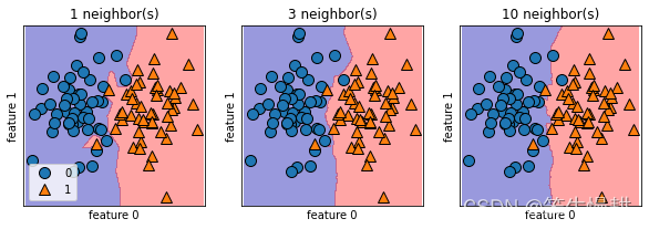

        如上图可知，在k=1决策边界精确地迎合两个类别的样本分布以犬牙交错的方式穿过整个样本空间，非如此不能得到100%的accuracy。而随着k值增大，决策边界则逐渐变得平缓，宁愿牺牲accuracy，也不会为了个别样本而绕出一条诡异的非规则曲线。这个决策边界的平滑度其实就直观地反映了模型复杂度，决策边界越平滑对应的模型就越简单。 

6. 优缺点

        优点：

        极其简单易懂，无需训练（训练过程其实就是训练集样本收集过程），可解释性高。在低维小数据集情况下是一个不错的算法。对异常值和噪声有较高的容忍度。

        缺点：

        计算复杂度高（计算量大，对内存需求高）。从算法原理可以看出，对每一个新的数据样本进行预测时，都要计算该样本与训练集中的所有样本的距离，并且进行排序。

        假设数据集的size为(m,n),即包含m个数据点，每个数据的维度为n，距离度量产生的时间复杂度为O(n),遍历数据集产生的时间复杂度为O(m),算法的时间复杂度为两者相乘O(mn)，另外，还有排序的时间复杂度大概为𝑂(𝑚𝑙𝑜𝑔𝑚))O(mlogm)).