4.1 多层感知机

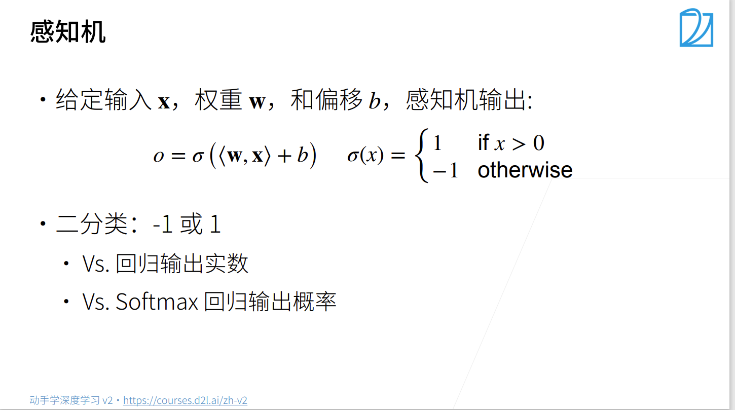
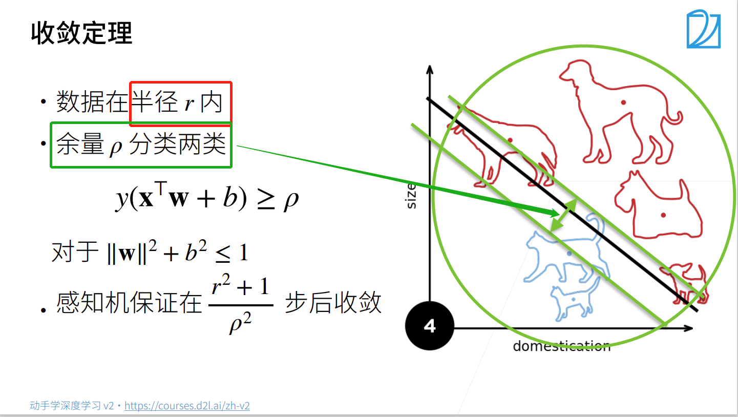
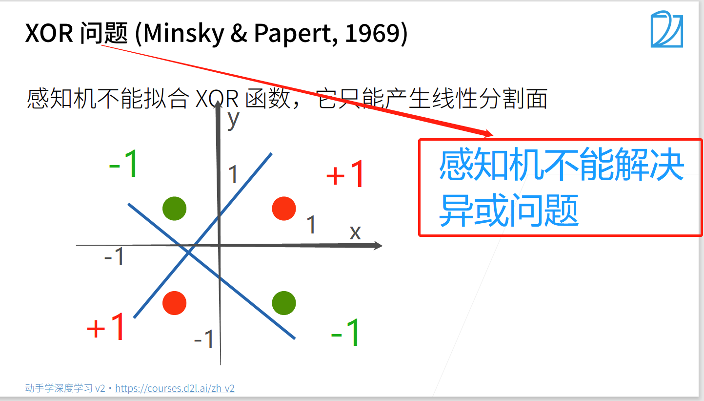
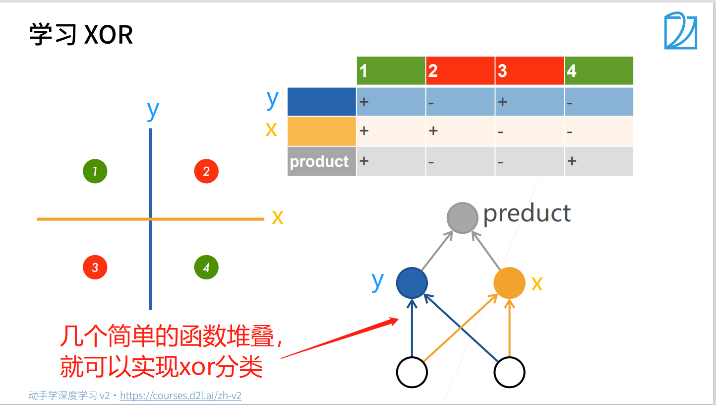
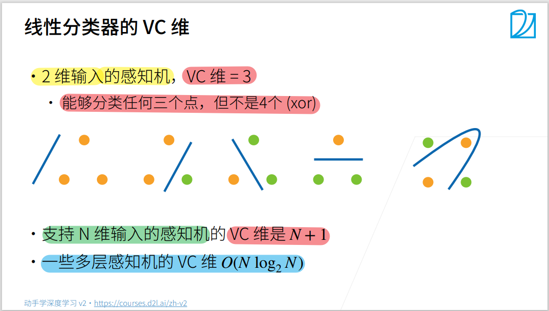
4.1.1 感知机

总结

• 感知机是一个二分类模型，是最早的模型之一
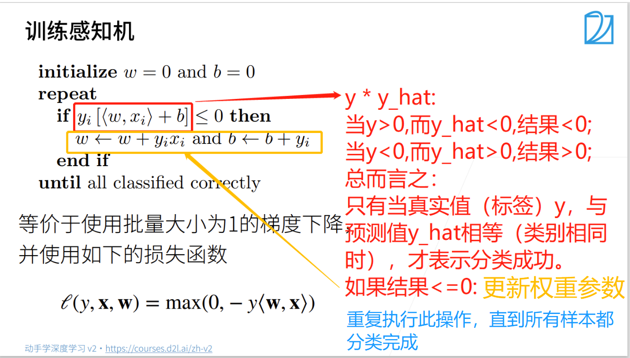
• 它的求解算法等价于使用批量大小为1的梯度下降
• 它不能拟合XOR函数，导致了第一次AI寒冬

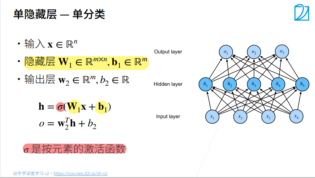
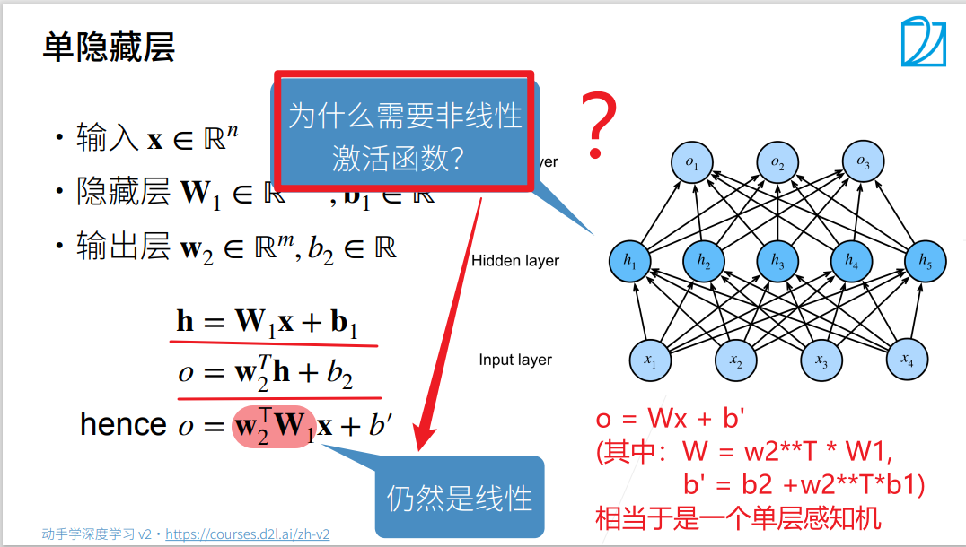
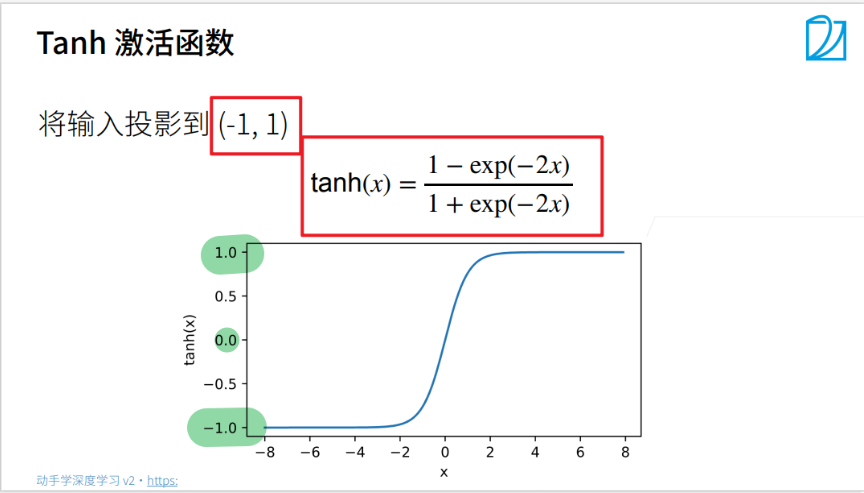
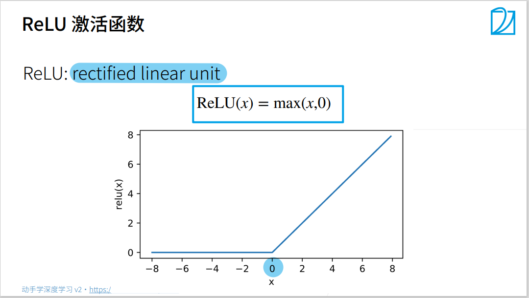
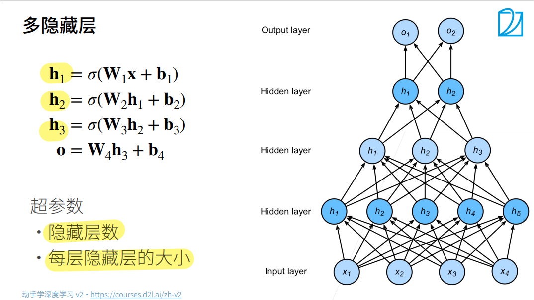
4.1.2 多层感知机

总结

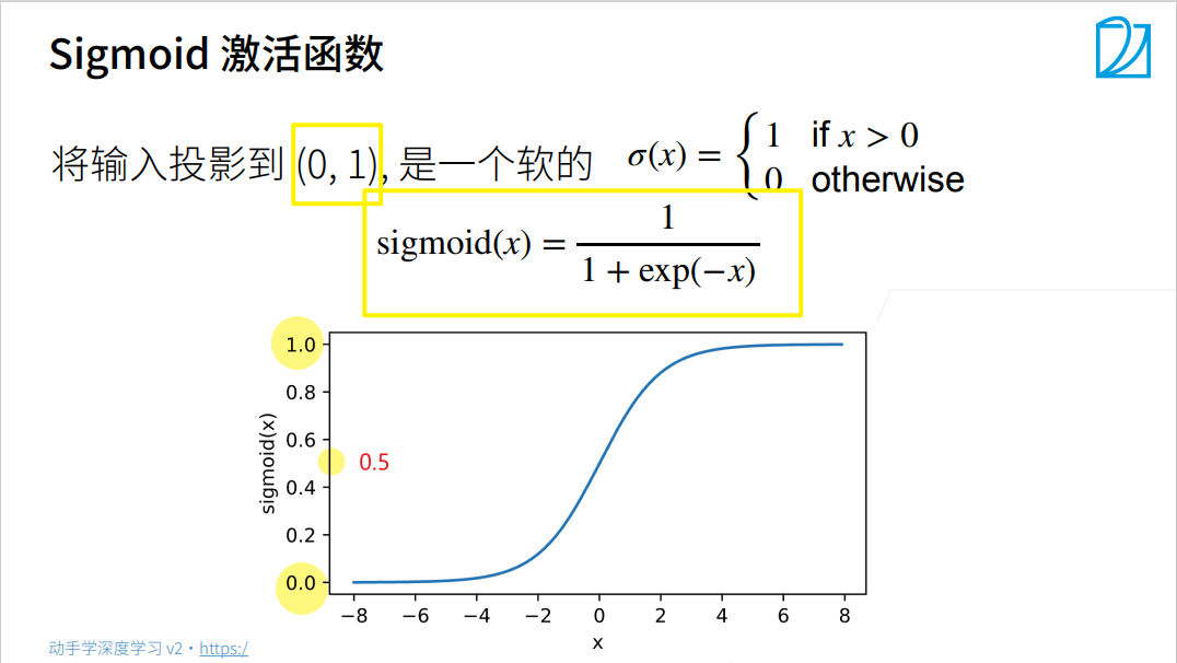
• 多层感知机使用隐藏层和激活函数来得到非线性模型
• 常用激活函数是Sigmoid， Tanh， ReLu
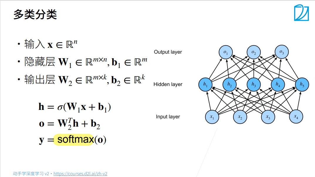
• 使用softmax来处理多分类
• 超参数为隐藏层数，和各个隐藏层大小

4.2 多层感知机的手动实现

导入相关库

import torch
from torch import nn
from d2l import torch as d2l

加载数据集

batch_size = 256
train_iter, test_iter = d2l.load_data_fashion_mnist(batch_size)

1. 初始化模型参数

实现一个具有单隐藏层的多层感知机，它包含256个隐藏单元

num_inputs, num_outputs, num_hiddens = 784, 10, 256

W1 = nn.Parameter(  # * 0.01：缩小权重张量的数值范围，可以避免梯度爆炸或消失，提高模型的稳定性和收敛速度
    torch.randn(num_inputs, num_hiddens, requires_grad=True) * 0.01)  # W1: [784, 256]
b1 = nn.Parameter(torch.zeros(num_hiddens, requires_grad=True))  # b1: [256]
W2 = nn.Parameter(
    torch.randn(num_hiddens, num_outputs, requires_grad=True) * 0.01)  # W2: [256, 10]
b2 = nn.Parameter(torch.zeros(num_outputs, requires_grad=True))  # b2: [10]

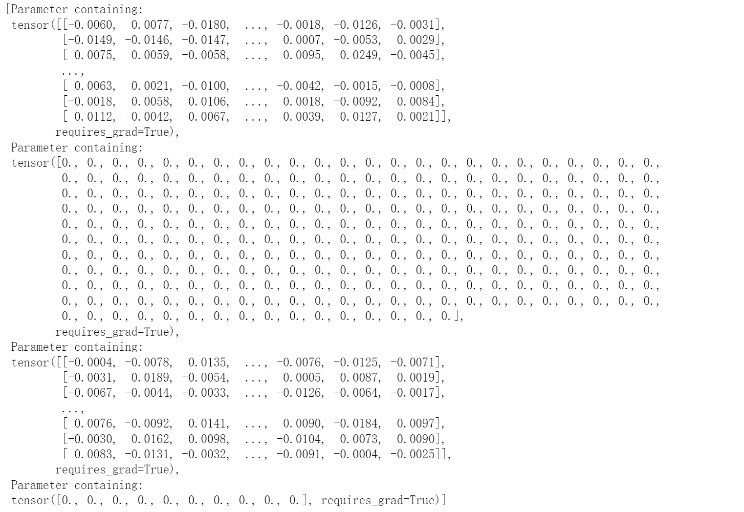
params = [W1, b1, W2, b2]

params

2. 定义激活函数

使用ReLU激活函数

def relu(X):
    a = torch.zeros_like(X)  # 张量形状与X相同，但是元素数值全为0
    return torch.max(X, a)

3. 定义模型

def net(X):
    X = X.reshape((-1, num_inputs))
    H = relu(X @ W1 + b1)  # X @ W1:矩阵乘法运算相当于 X.mm(W1)，X.matmul(W1)
    return H @ W2 + b2

4. 定义损失函数

loss = nn.CrossEntropyLoss(reduction='none')

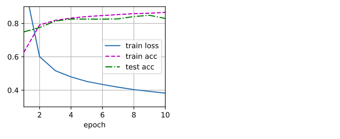
5. 训练

（训练效果上， 相较于softmax，loss降低了， 但是精度并没有上升很多）

num_epochs, lr = 10, 0.1
updater = torch.optim.SGD(params, lr=lr)
d2l.train_ch3(net, train_iter, test_iter, loss, num_epochs, updater)

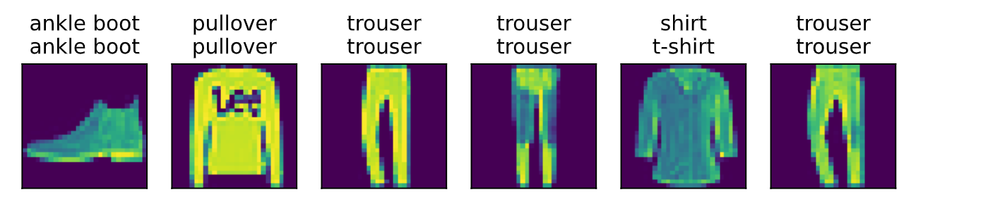
6. 预测

d2l.predict_ch3(net, test_iter)

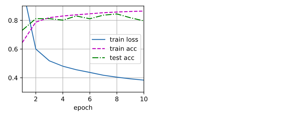
4.3 多层感知机的简洁实现

• 相较于手动实现，就模型用的是nn模块， 其余部分均一样

1. 定义模型

net = nn.Sequential(
    nn.Flatten(),
    nn.Linear(784, 256),
    nn.ReLU(),
    nn.Linear(256, 10))

2. 初始化模型参数

def init_weights(m):
    if type(m) == nn.Linear:
        nn.init.normal_(m.weight, std=0.01)

net.apply(init_weights)### 4.2.1 初始化模型参数

3. 定义各种超参数

batch_size, lr, num_epochs = 256, 0.1, 10
loss = nn.CrossEntropyLoss(reduction='none')
trainer = torch.optim.SGD(net.parameters(), lr=lr)

4. 训练

train_iter, test_iter = d2l.load_data_fashion_mnist(batch_size)
d2l.train_ch3(net, train_iter, test_iter, loss, num_epochs, trainer)### 4.2.1 初始化模型参数

4.4 模型选择

4.4.1 训练误差和泛化误差

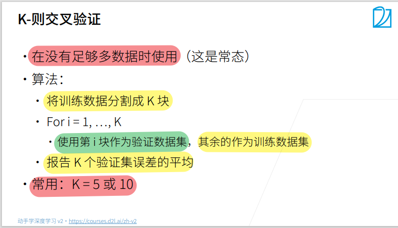
4.4.2 模型选择

总结

• 训练数据集：训练模型参数
• 验证数据集：选择模型超参数
• 非大数据集上通常使用K-折交叉验证

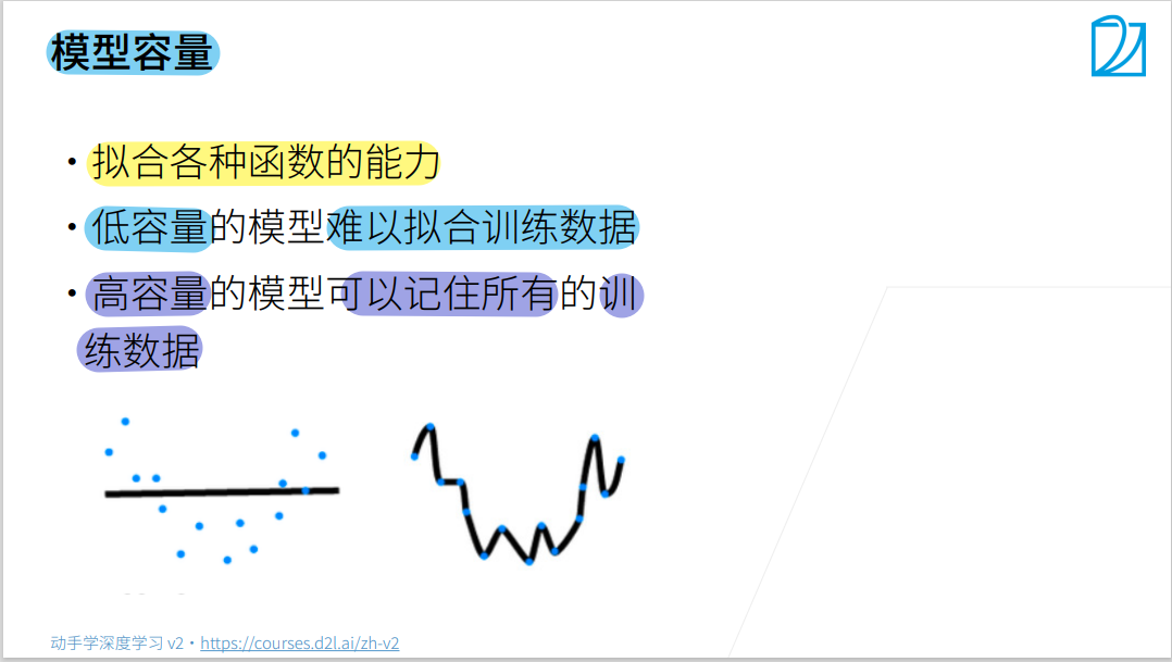
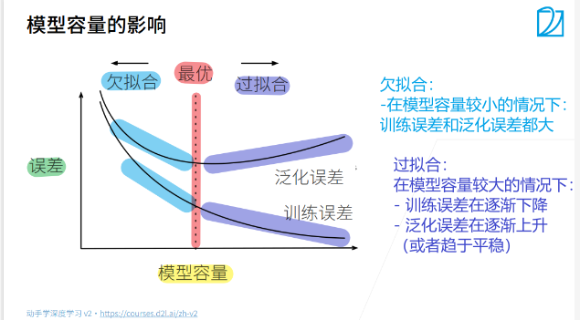
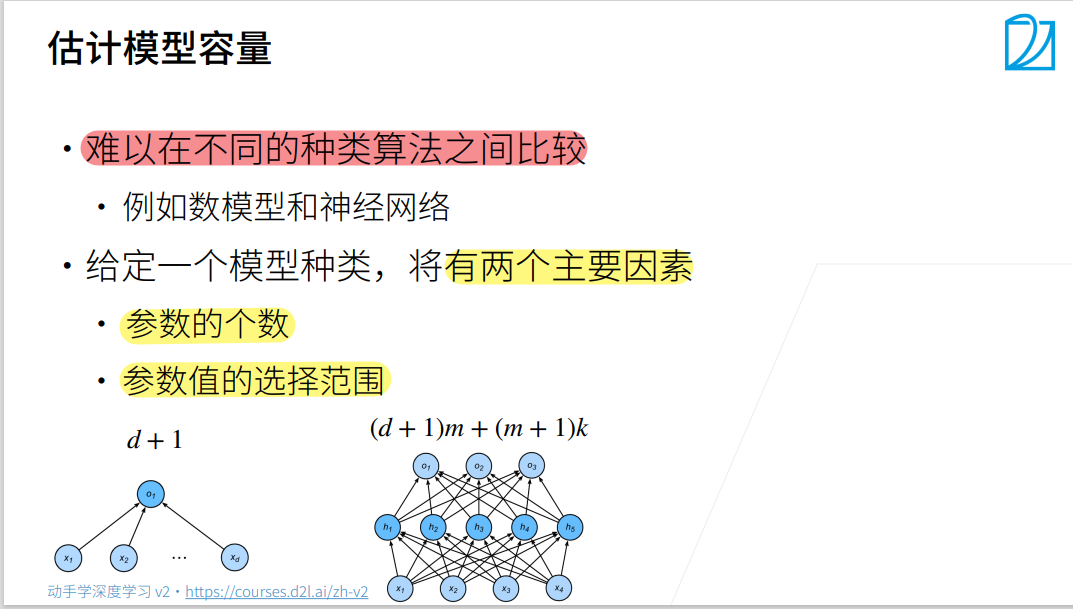
4.4.3 过拟合和欠拟合

总结

• 模型容量需要匹配数据复杂度， 否则可能导致欠拟合和过拟合
• 统计学习提供数据工具来衡量模型复杂度
• 实际中一般靠观察训练误差和验证误差

4.4.4 多项式回归

0. 导入相关库

import math
import numpy as np
import torch
from torch import nn
from d2l import torch as d2l

1. 生成数据集
   给定x, 使用以下三阶多项式来生成训练数据和测试数据的标签：
   
   PyTorch中的两类乘法

max_degree = 20  # 多项式的最大阶数
n_train, n_test = 100, 100  # 训练数据集和测试数据集的大小
true_w = np.zeros(max_degree)  # 给权重w分配大量的空间  # w[20]
true_w[0: 4] = np.array([5, 1.2, -3.4, 5.6])

features = np.random.normal(size=(n_train + n_test, 1)) 
# features[200, 1]：元素为均值为0，标准差为1的正态分布
np.random.shuffle(features)
poly_features = np.power(
	features, np.arange(max_degree).reshape(1, -1))  # poly_features[200, 20] 
for i in range(max_degree):
    poly_features[:, i] /= math.gamma(i + 1)  # gamma(n) = (n-1)!
# labels的维度：（n_train + n_test, )
labels = np.dot(poly_features, true_w)  # [200,20] , [20] = [200,]
labels += np.random.normal(scale=0.1, size=labels.shape)  # labels = labels + 噪声

# NumPyndarray 转换为tensor
true_w, features, poly_features, labels = [torch.tensor(x, dtype=torch.float32) 
                                           for x in [true_w, features, poly_features, labels]]

features[:2], poly_features[:2, :], labels[:2]

2. 对模型进行训练和测试
实现一个函数来评估模型在给定数据集上的损失

def evaluate_loss(net, data_iter, loss):
    """评估给定数据集上模型的损失"""
    metric = d2l.Accumulator(2)  # 损失的总和，样本数量
    for X, y in data_iter:
        out = net(X)
        y = y.reshape(out.shape)
        l = loss(out, y)
        metric.add(l.sum(), l.numel())
    return metric[0] / metric[1]

定义训练函数

def train(train_features, test_features, train_labels, test_labels, 
          num_epochs=400):
    loss = nn.MSELoss(reduction='none')
    input_shape = train_features.shape[-1]
    # 不设置偏置， 因为已经在多项式中实现了它
    net = nn.Sequential(
        nn.Linear(input_shape, 1, bias=False))
    batch_size = min(10, train_labels.shape[0])
    train_iter = d2l.load_array((train_features, train_labels.reshape(-1, 1)),
                                batch_size)
    test_iter = d2l.load_array((test_features, test_labels.reshape(-1, 1)),
                               batch_size, is_train=False)
    trainer = torch.optim.SGD(net.parameters(), lr=0.01)
    animator = d2l.Animator(xlabel='epoch', ylabel='loss', yscale='log',
                            xlim=[1, num_epochs], ylim=[1e-3, 1e2],
                            legend=['train', 'test'])
    for epoch in range(num_epochs):
        d2l.train_epoch_ch3(net, train_iter, loss, trainer)
        if epoch == 0 or (epoch + 1) % 20 == 0:
            animator.add(epoch + 1, (evaluate_loss(net, train_iter, loss),
                                     evaluate_loss(net, test_iter, loss)))
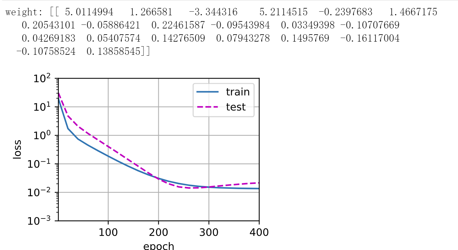
    print('weight:', net[0].weight.data.numpy())

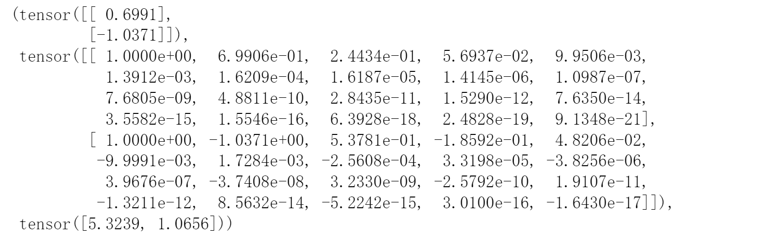
3. 三阶多项式函数拟合（正常）

# 从多项式特征中选择前4个维度: 1、x、x^2/2!和x^3/3!
train(poly_features[:n_train, :4], poly_features[n_train:, :4],
      labels[:n_train], labels[n_train:])

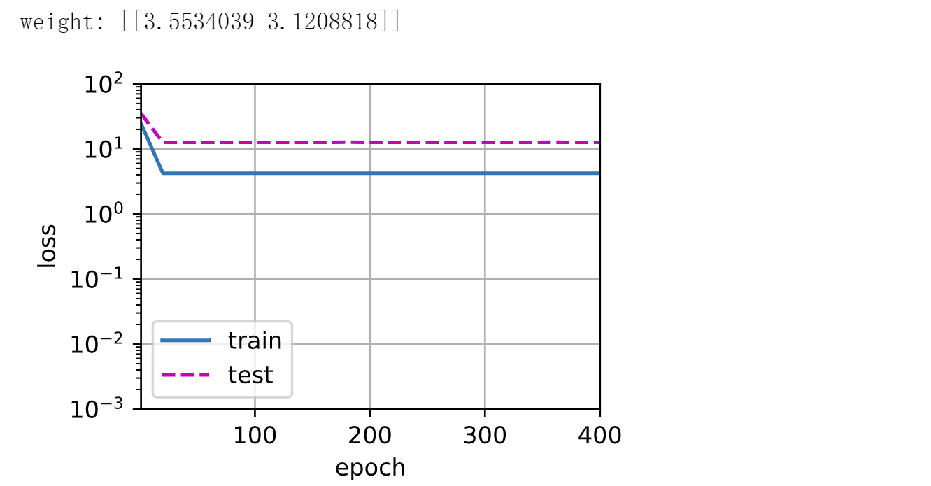
4. 线性函数拟合（欠拟合）

# 从多项式特征中选择前两个维度，即1和X
train(poly_features[:n_train, :2], poly_features[n_train:, :2],
      labels[:n_train], labels[n_train:])

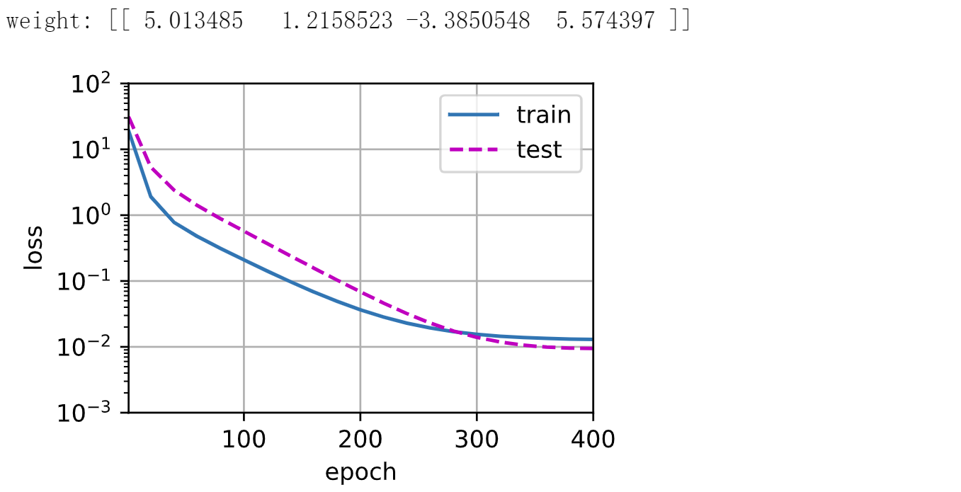
5. 高阶多项式函数拟合（过拟合）

# 从多项式特征中选取所有维度
train(poly_features[:n_train, :], poly_features[n_train:, :],
      labels[:n_train], labels[n_train:])

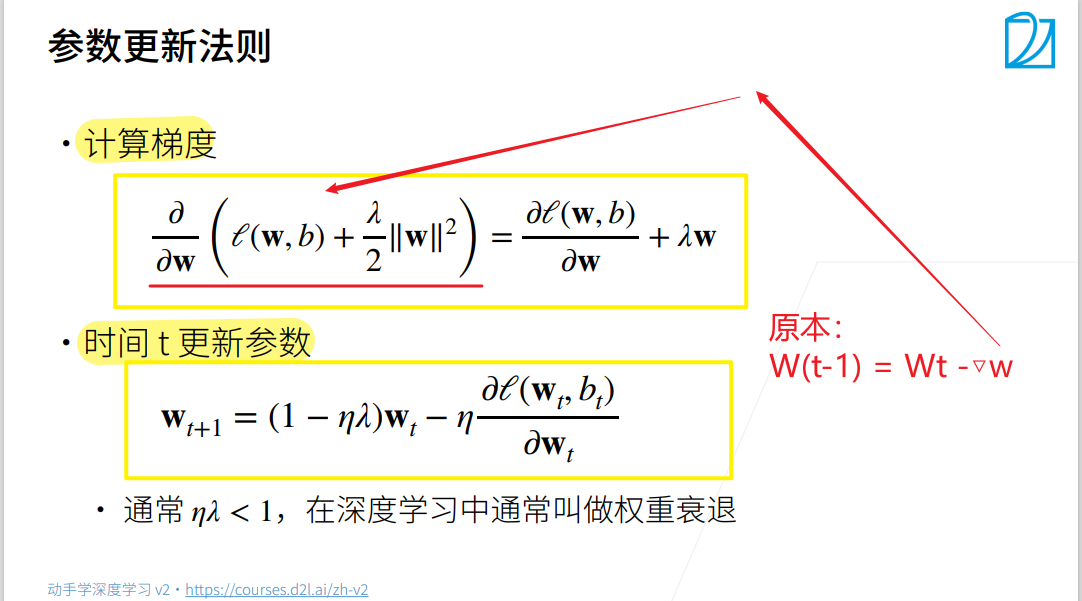
4.5 权重衰退(L2正则化)

4.5.1 范数与权重衰减

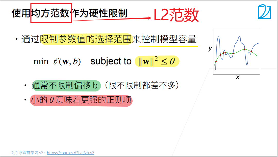
为什么使用$L_2$范数来进行正则化，而不是使用$L_1$范数？

• $L_2$正则化线性模型构成经典的岭回归（ridge regression）算法，
• $L_1$正则化线性回归是统计学中类似的基本模型， 通常被称为套索回归（lasso regression）。
• 使用L2范数的一个原因是它对权重向量的大分量施加了巨大的惩罚。 这使得我们的学习算法偏向于在大量特征上均匀分布权重的模型。 在实践中，这可能使它们对单个变量中的观测误差更为稳定。
• 相比之下，$L_1$惩罚会导致模型将权重集中在一小部分特征上， 而将其他权重清除为零。 这称为特征选择（feature selection），这可能是其他场景下需要的

总结

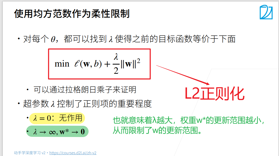
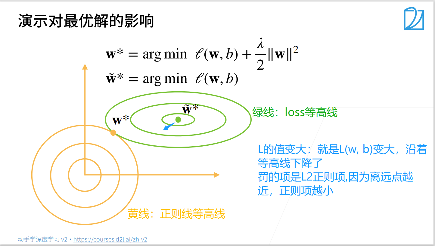
• 权重衰退通过$L_2$正则化使得模型参数不会过大， 从而控制模型复杂度
• 正则项权重是控制模型复杂度的超参数

4.5.2 高维线性回归

%matplotlib inline
import torch
from torch import nn
from d2l import torch as d2l

生成数据：
$y=0.05+{\sum }_{i=1}^{d}0.01x_i+€$ where € ～ N(0, $0.01^2$)

n_train, n_test, num_inputs, batch_size = 20, 100, 200, 5  # 训练数据较小，很容易过拟合
true_w, true_b = torch.ones((num_inputs, 1)) * 0.01, 0.05
train_data = d2l.synthetic_data(true_w, true_b, n_train)  # Generate y = Xw + b + noise
train_iter = d2l.load_array(train_data, batch_size)  # Construct a PyTorch data iterator
test_data = d2l.synthetic_data(true_w, true_b, n_test)
test_iter = d2l.load_array(test_data, batch_size, is_train=False)  # shuffle=is_train :是否随机打乱

4.5.3 权重衰减的手动实现

1. 初始化模型参数

def init_params():
    w = torch.normal(0, 1, size=(num_inputs, 1), requires_grad=True)
    b = torch.zeros(1, requires_grad=True)
    return [w, b]

2. 定义$L_2$范数惩罚

def l2_penalty(w):
    return torch.sum(w.pow(2)) / 2  # L2范数
#     return torch.sum(torch.abs(w)) # L1范数

3. 定义训练函数

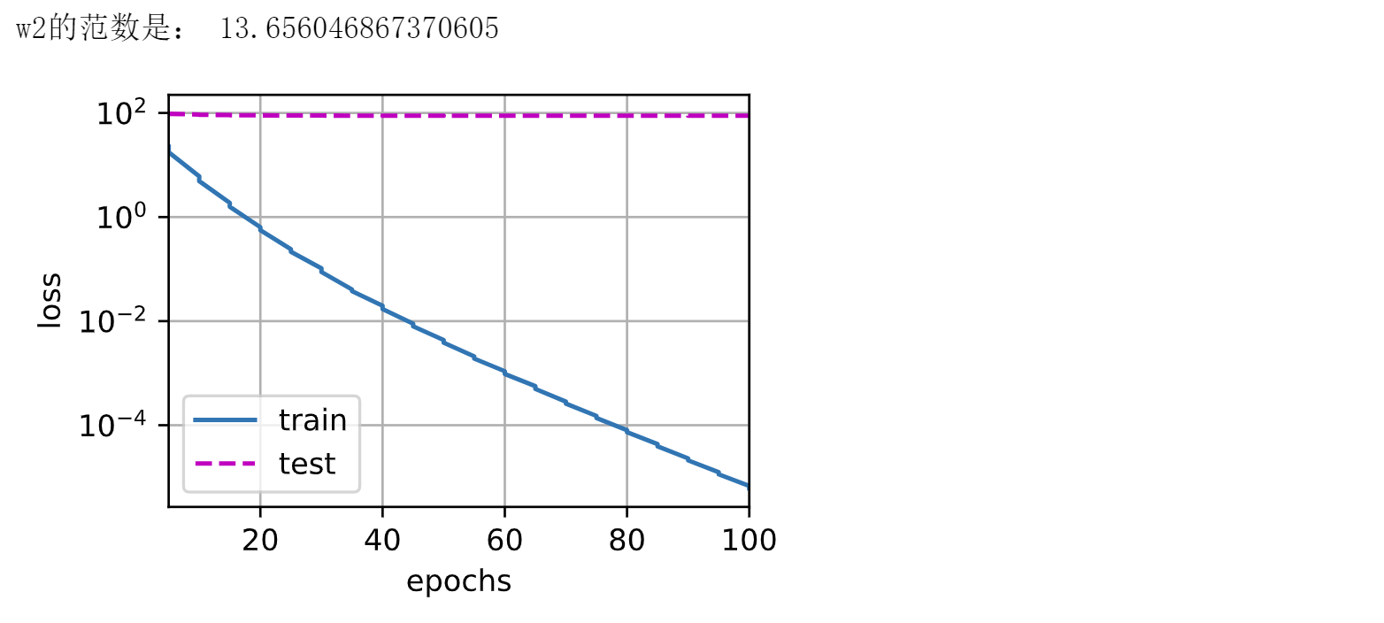
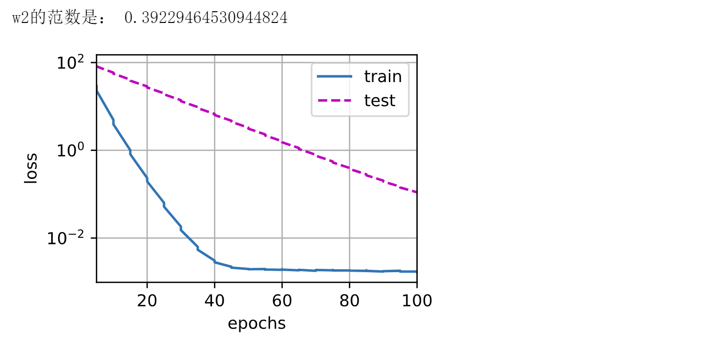
def train(lambd):
    w, b = init_params()
    net, loss = lambda X: d2l.linreg(X, w, b), d2l.squared_loss
    num_epochs, lr = 100, 0.003
    animator = d2l.Animator(xlabel='epochs', ylabel='loss', yscale='log',
                            xlim=[5, num_epochs], legend=['train', 'test'])
    for epoch in range(num_epochs):
        for X, y in train_iter:
            # with torch.enable_grad():  允许计算梯度
            # 增加了L2范数惩罚项
            # 广播机制l2_penalty(w)成为一个长度为batch_size的向量
            l = loss(net(X), y) + lambd * l2_penalty(w)
            l.sum().backward()
            d2l.sgd([w, b], lr, batch_size)
            if (epoch + 1) % 5 == 0:
                animator.add(epoch + 1, (d2l.evaluate_loss(net, train_iter, loss),
                                         d2l.evaluate_loss(net, test_iter, loss)))
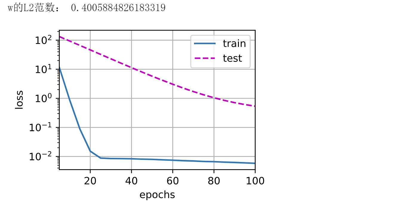
    print('w2的范数是：', torch.norm(w).item())

4. 忽略正则化，直接训练

train(lambd=0)  # 忽略正则化直接训练

5. 使用正则化，训练

train(lambd=3)  # 使用权重衰减

4.5.4 权重衰减的简洁实现

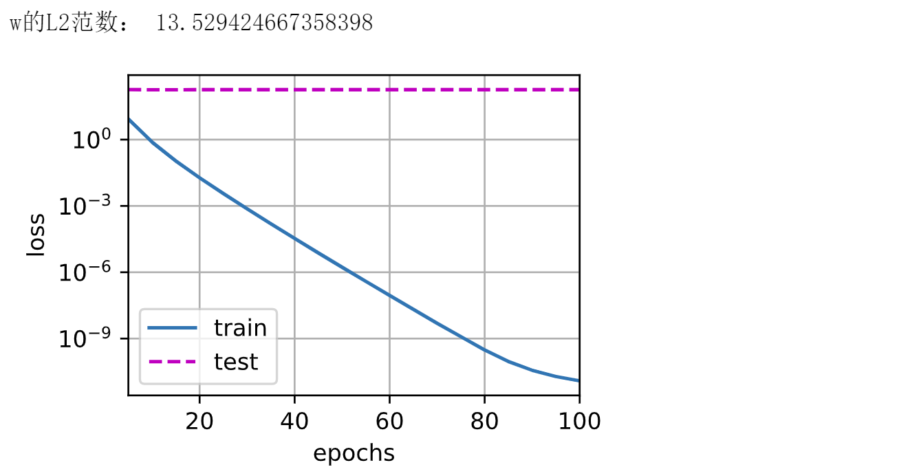
def train_concise(wd):
    net = nn.Sequential(
        nn.Linear(num_inputs, 1))
    for param in net.parameters():
        param.data.normal_()
    loss = nn.MSELoss(reduction='none')
    num_epochs, lr = 100, 0.003
    # 偏置参数没有衰减
    trainer = torch.optim.SGD([{"params": net[0].weight, 'weight_decay': wd},
                               {"params": net[0].bias}], lr=lr)
    animator = d2l.Animator(xlabel='epochs', ylabel='loss', yscale='log',
                            xlim=[5, num_epochs], legend=['train', 'test'])

    for epoch in range(num_epochs):
        for X, y in train_iter:
            trainer.zero_grad()
            l = loss(net(X), y)
            l.mean().backward()
            trainer.step()
        if (epoch + 1) % 5 == 0:
            animator.add(epoch + 1,
                         (d2l.evaluate_loss(net, train_iter, loss),
                          d2l.evaluate_loss(net, test_iter, loss)))
    print("w的L2范数：", net[0].weight.norm().item())

train_concise(0)  # 忽略正则化直接训练

train_concise(3)  # 使用权重衰减

4.6 暂退法(Dropout)

4.6.1 暂退法

总结

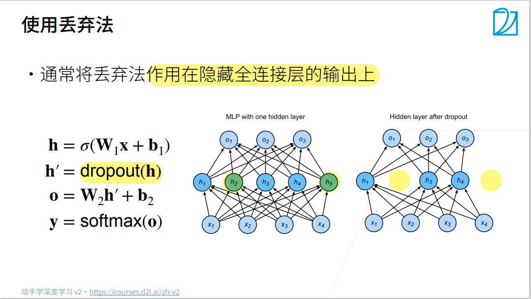
• 丢弃法将一些输出项随机置0来控制模型复杂度
• 常作用在多层感知机的隐藏层输出上
• 丢弃概率是控制模型复杂度的超参数
• 常用技巧：在靠近输入的地方设置较低的暂退概率

4.6.2 Dropout的手动实现

1. 导入相关库

import torch
from torch import nn
from d2l import torch as d2l

2. 定义Dropout函数

def dropout_layer(X, dropout):
    assert 0 <= dropout <= 1
    if dropout == 1:
        return torch.zeros_like(X)
    if dropout == 0:
        return X
    mask = (torch.rand(X.shape) > dropout).float()
    return mask * X / (1.0 - dropout)  # 不用X[mask] = 0：对于cpu和gpu做乘法比选择快很多

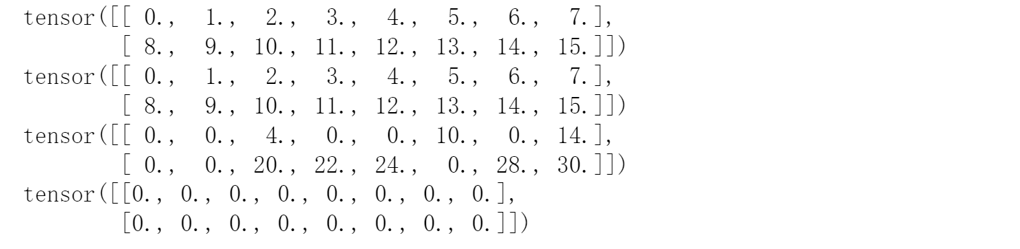
X = torch.arange(16, dtype=torch.float32).reshape(2, 8)
print(X)
print(dropout_layer(X, 0.))
print(dropout_layer(X, 0.5))
print(dropout_layer(X, 1.))

3. 定义模型参数

• 模型有两个隐藏层，每个隐藏层包含256个隐藏单元
• 靠近输入层的地方dropout设置较低的暂退概率

num_inputs, num_outputs, num_hidden1, num_hidden2 = 784, 10, 256, 256
dropout1, dropout2 = 0.2, 0.5

4. 定义模型

class Net(nn.Module):
    def __init__(self, num_inputs, num_outputs, num_hidden1, num_hidden2, is_training=True):
        super(Net,self).__init__()
        self.num_inputs = num_inputs
        self.training = is_training
        self.lin1 = nn.Linear(num_inputs, num_hidden1)
        self.lin2 = nn.Linear(num_hidden1, num_hidden2)
        self.lin3 = nn.Linear(num_hidden2, num_outputs)
        self.relu = nn.ReLU()

    def forward(self, X):
        H1 = self.relu(self.lin1(X.reshape(-1, self.num_inputs)))
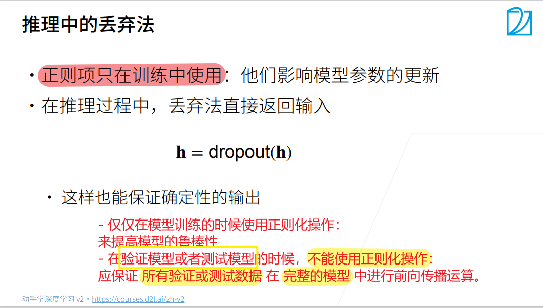
        # 只有在训练模型时才使用暂退法
        if self.training:
            # 在第一个全连接层之后添加一个暂退层
            H1 = dropout_layer(H1, dropout1)
        H2 = self.relu(self.lin2(H1))
        if self.training:
            H2 = dropout_layer(H2, dropout2)
        out = self.lin3(H2)
        return out

net = Net(num_inputs, num_outputs, num_hidden1, num_hidden2)
net

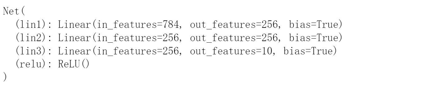
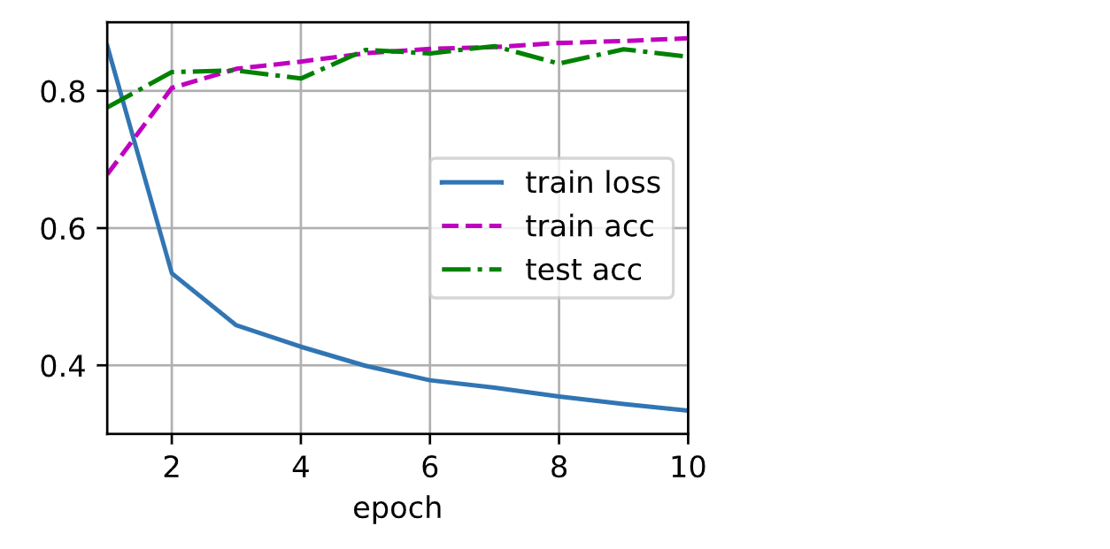
5. 训练

num_epochs, lr, batch_size = 10, 0.5, 256
loss = nn.CrossEntropyLoss(reduction='none')
train_iter, test_iter = d2l.load_data_fashion_mnist(batch_size)
trainer = torch.optim.SGD(net.parameters(), lr=lr)
d2l.train_ch3(net, train_iter, test_iter, loss, num_epochs, trainer)

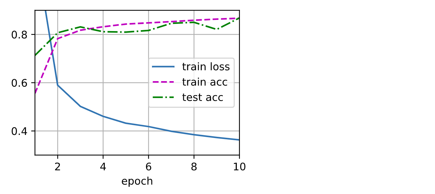
4.6.1 Dropout的简洁实现

1. 导入相关库

import torch
from torch import nn
from d2l import torch as d2l

2. 设置dropout概率

dropout1, dropout2 = 0.3, 0.5

3. 定义模型

net = nn.Sequential(
    nn.Flatten(),
    nn.Linear(784, 256), nn.ReLU(),
    # 在第一个全连接层之后添加一个暂退层
    nn.Dropout(dropout1),
    nn.Linear(256, 256), nn.ReLU(),
    # 在第二个全连接层之后添加以一个暂退层
    nn.Dropout(dropout2),
    nn.Linear(256, 10))


def init_weight(m):
    if type(m) == nn.Linear:
        nn.init.normal_(m.weight, std=0.01)

net.apply(init_weight)

4. 定义超参数

num_epochs, lr, batch_size = 10, 0.5, 256
loss = nn.CrossEntropyLoss(reduction='none')
train_iter, test_iter = d2l.load_data_fashion_mnist(batch_size)
trainer = torch.optim.SGD(net.parameters(), lr=lr)

5. 训练

d2l.train_ch3(net, train_iter, test_iter, loss, num_epochs, trainer)

4.7 数值稳定性与模型初始化

4.7.1 数值稳定性

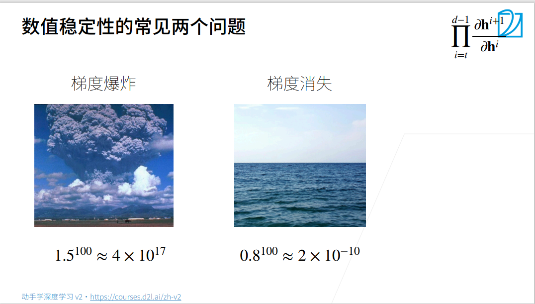
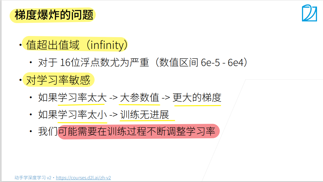
总结

• 当数值过大或者过小时导致数值问题
• 常发生在深度模型中，通常会对n个数累乘。

4.7.2 模型初始化与常用激活函数

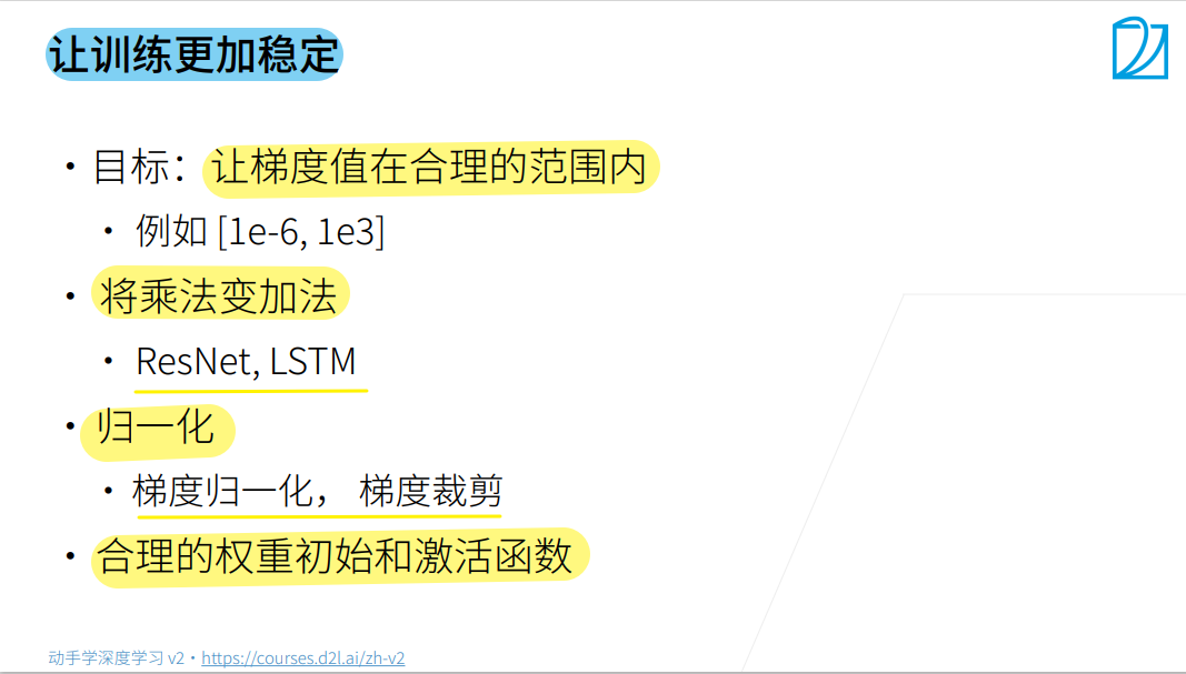
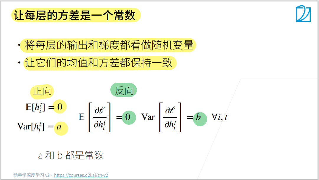
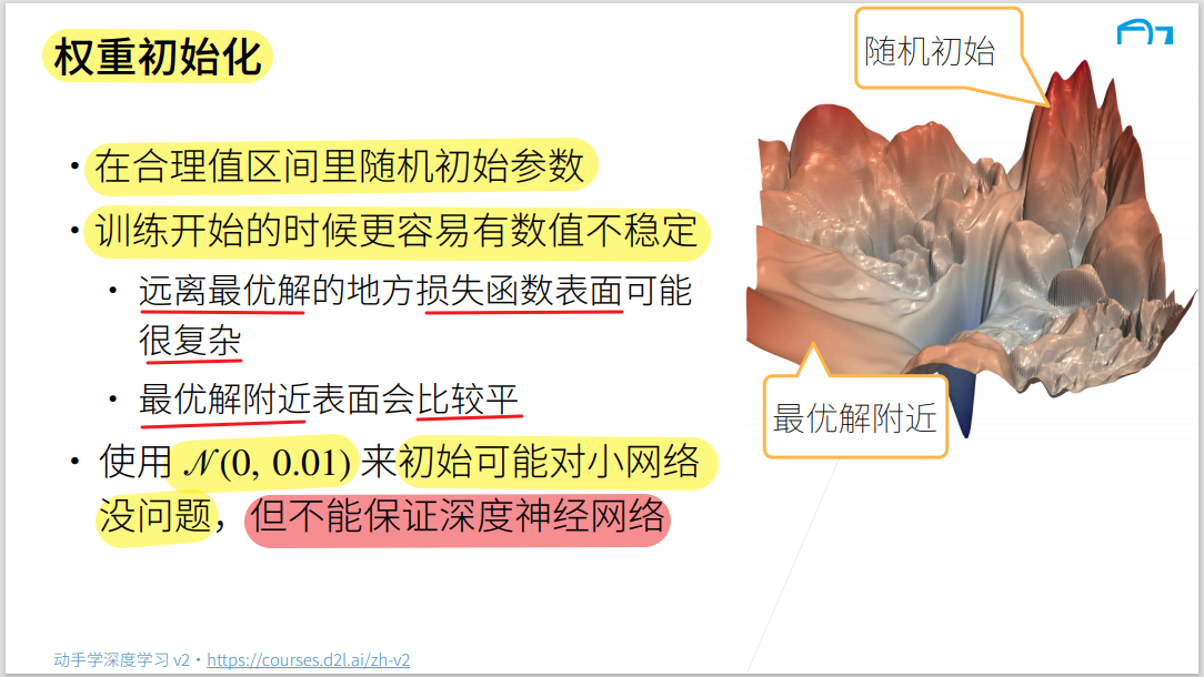
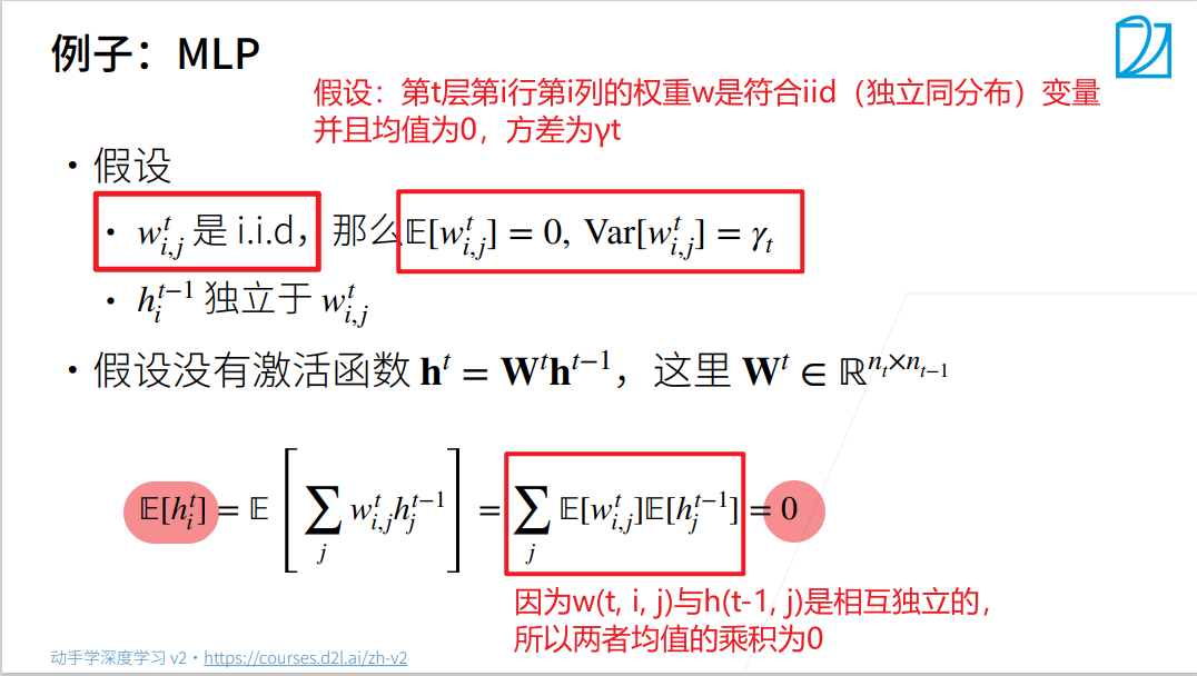
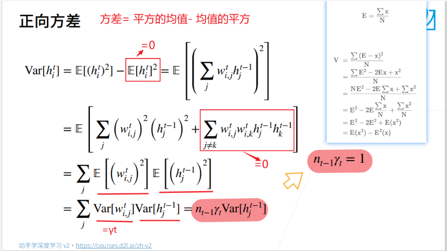
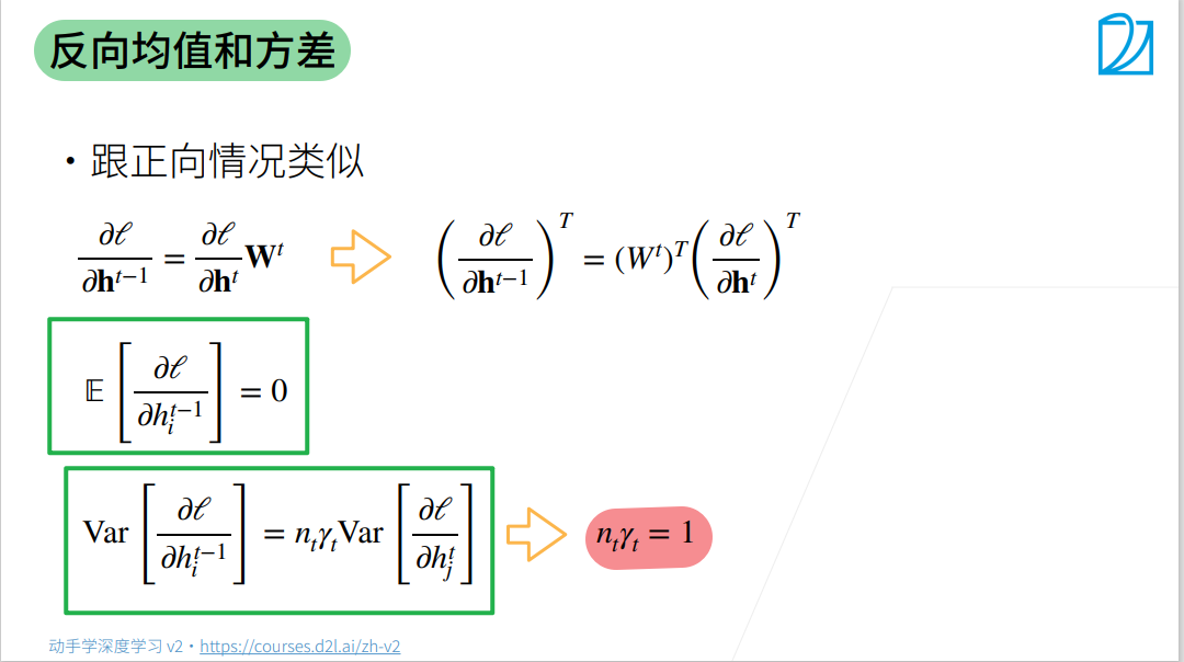
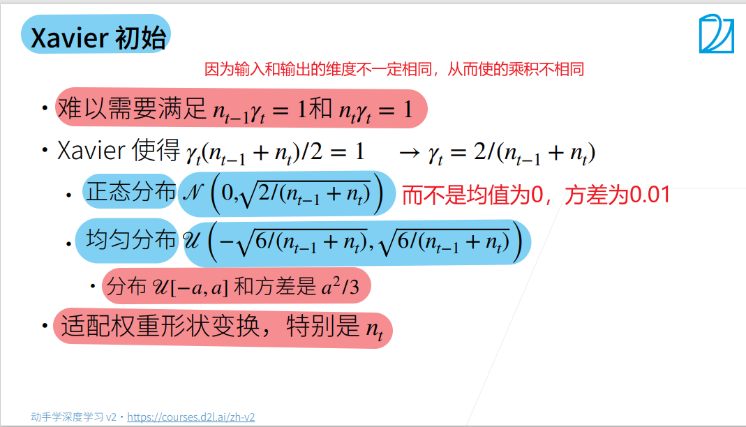
总结

• 合理的权重初始值和激活函数的选取可以提升数值稳定性

4.8 实战kaggle比赛：预测房价

hashlib库与requests库

1. hashlib库中的SHA1加密函数

SHA1加密（安全哈希算法）（Secure Hash Algorithm）：主要适用于数字签名标准（Digital Signature
Standard DSS）里面定义的数字签名算法（Digital Signature Algorithm
DSA），SHA1比MD5的安全性更强。对于长度小于2^ 64位的消息，SHA1会产生一个160位的消息摘要。

链接：更多加密算法
链接：hashlib的用法

# SHA1加密用法
import hashlib                      # 1. 在python中引用hashlib模块
sha1 = hashlib.sha1()               # 2. 创建一个hash对象，使用hash算法命名的构造函数，或者通用构造函数
data = '2333333'  
sha1.update(data.encode('utf-8'))   # 3. 使用hash对象调用update()方法填充对象
sha1_data = sha1.hexdigest()        # 4. 调用digest()（字节对象）或者hexdigest()（字符串对象）方法来获取摘要（加密结果）
print(sha1_data)

2. requests库中的get()函数

• requests.get()：用Python像浏览器一样发送Get/Post请求,

• stream=False（默认），他会立即开始下载文件并存放到内存当中，倘若文件过大就会导致内存不足的情况。

• stream参数设置成True时，它不会立即开始下载，当你使用iter_content或iter_lines遍历内容或访问内容属性时才开始下载。

• • 需要注意一点：文件没有下载之前，它也需要保持连接。这里就用到了另一个巧妙的库了:
• • contextlib.closingiter_content：一块一块的遍历要下载的内容
• • iter_lines：一行一行的遍历要下载的内容，
    使用上面两个函数下载大文件可以防止占用过多的内存，因为每次只下载小部分数据。

• verify=True(默认): 检查证书认证

• verify=False(常用): 忽略证书认证

链接：requests的用法
链接：requests 中的参数stream
链接：参数stream=True的含义
链接：request.get()参数详解

导入相关库

import hashlib  # 1. 引用hashlib模块
import os
import tarfile
import zipfile
import requests  # requests是使用Apache2 licensed 许可证的HTTP库

1. 下载和缓存数据集

DATA_HUB = dict()
DATA_URL = 'http://d2l-data.s3-accelerate.amazonaws.com/'

def download(name, cache_dir=os.path.join('..', 'data')):
    """下载一个DATA_HUB中的文件，返回本地文件名。"""
    assert name in DATA_HUB, f'{name}不在于{DATA_HUB}.'
    url, sha1_hash = DATA_HUB[name]
    os.makedirs(cache_dir, exist_ok=True)
    fname = os.path.join(cache_dir, url.split('/')[-1])
    if os.path.exists(fname):
        sha1 = hashlib.sha1()  # 2. 调用加密函数来创建对象
        with open(fname, 'rb') as f:
            while True:
                data = f.read(1048576)  # 是HDFS默认的一个参数：默认是1048576：每次读取1048576字节，也就是1MB
                if not data:
                    break
                sha1.update(data)  # 调用update()方法填充对象
        if sha1.hexdigest() == sha1_hash:  # hexdigest()（字符串对象）方法来获取摘要
            return fname  # 命中缓存
    print(f'正在从{url}下载{fname}...')
    r = requests.get(url, stream=True, verify=True)
    with open(fname, 'wb') as f:
        f.write(r.content)
    return fname

def download_extract(name, folder=None):
    """下载并解压zip/tar文件"""
    fname = download(name)
    base_dir = os.path.dirname(name)
    data_dir, ext = os.path.splitext(fname)
    if ext == '.zip':
        fp = zipfile.ZipFile(fname, 'r')
    elif ext in ('.tar', '.gz'):
        fp = tarfile.open(fname, 'r')
    else:
        assert False, '只有zip/tar文件可以被解压缩'
    fp.extractall(base_dir)
    return os.path.join(base_dir, folder) if folder else data_dir

def download_all():
    """下载DATA_HUB中的所有文件"""
    for name in DATA_HUB:
        download(name)

2. 访问和读取数据集

• 使用pandas读入并处理数据

%matplotlib inline
import numpy as np
import pandas as pd
import torch
from torch import nn
from d2l import torch as d2l

DATA_HUB['kaggle_house_train'] = (  # @save
    DATA_URL + 'kaggle_house_pred_train.csv',
    '585e9cc93e70b39160e7921475f9bcd7d31219ce')

DATA_HUB['kaggle_house_test'] = (  # @save
    DATA_URL + 'kaggle_house_pred_test.csv',
    'fa19780a7b011d9b009e8bff8e99922a8ee2eb90')

train_data = pd.read_csv(download('kaggle_house_train'))
test_data = pd.read_csv(download('kaggle_house_test'))

print(train_data.shape)
print(test_data.shape)

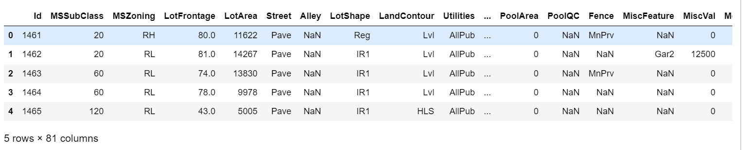
train_data.head()

test_data.head()

查看训练集中的前四个和最后两个特征， 以及相关标签(房价)
Pandas中loc和iloc函数（提取某几列或者行的数据）

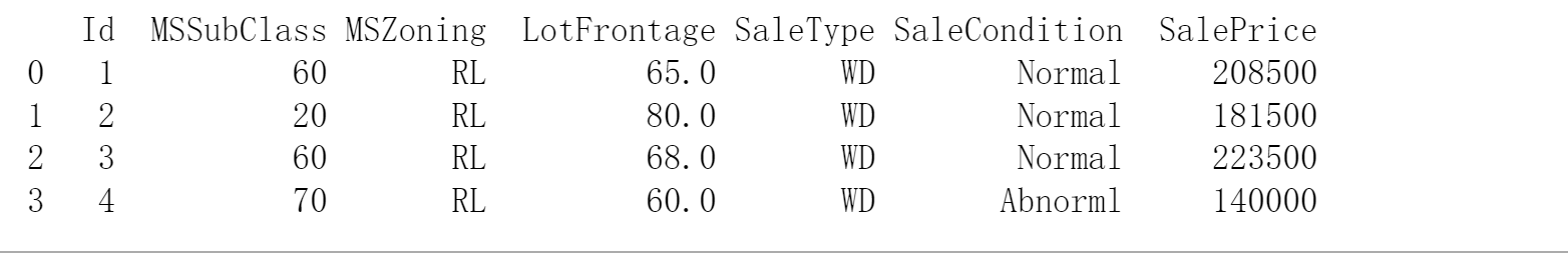
print(train_data.iloc[0:4, [0, 1, 2, 3, -3, -2, -1]])

在每个样本中，第一个特征是ID，我们将其从数据集中删除，并将测试集的最后一列（标签）也删除

# 列表中的[1:-1] 表示从第二个元素开始到倒数第二个元素结束，[左闭, 右开）
all_features = pd.concat((train_data.iloc[:, 1:-1], test_data.iloc[:, 1:]))

all_features.shape  # 81-2=79, 80-1=79

3. 数据集预处理

(1). 处理数值型数据

• 首先，将所有特征缩放到均值为0， 方差为1的正态分布，来标准化数据：（x - x.均值）/ x.标准差
• 然后，将所有缺失值替换为相应特征的平均值，即缺失值设置为0(来保证整个特征的均值是0，方差为1)

# 若无法获得测试数据，可根据训练数据计算均值和标准差
# 取出特征为数值型的所有列
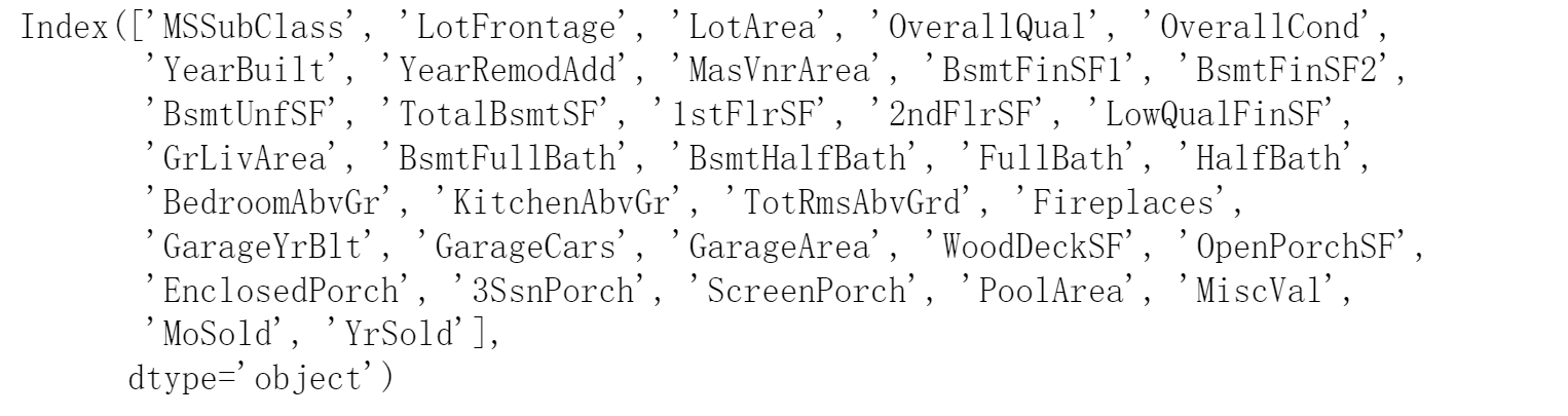
numeric_features = all_features.dtypes[all_features.dtypes != 'object'].index 
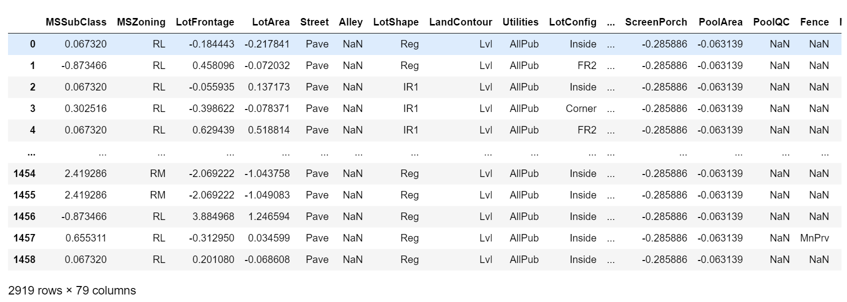
all_features[numeric_features] = all_features[numeric_features].apply(
    lambda x: (x - x.mean()) / (x.std()))
# 在标准化数据后，所有均值消失，因此我们可以将缺失值设置为0
all_features[numeric_features] = all_features[numeric_features].fillna(0)

numeric_features

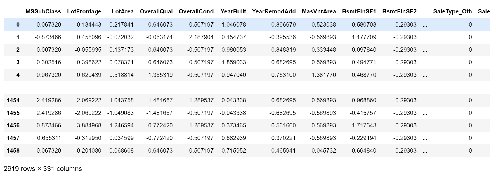
all_features

(2). 处理离散型数据

• 用一次独热编码替换它们

# dummy_na=True将na(缺失值)视为有效的特征值，并为其创建指示符特征
all_features = pd.get_dummies(all_features, dummy_na=True)
all_features.shape

all_features

(3). 数据类型转换

• 将样本中所有特征值从pandas格式中的ndarray格式转换成tensor，并将其数据类型设为float32。

n_train = train_data.shape[0]  # train_data.shape:[1460, 81]   train_data.shape[0]:1460
train_features = torch.tensor(all_features[:n_train].values, dtype=torch.float32)
test_features = torch.tensor(all_features[n_train:].values, dtype=torch.float32)
train_labels = torch.tensor(train_data.SalePrice.values.reshape(-1, 1), dtype=torch.float32)

train_features.shape, test_features.shape, train_labels.shape

4. 构建模型

定义损失函数和特征维数

loss = nn.MSELoss()
in_features = train_features.shape[1]

定义网络模型

def get_net():
    net = nn.Sequential(
    nn.Linear(in_features, 1))  # 331--->1
    return net

定义损失函数

我们更关心相对误差(y-y_hat)/y（=1-y_hat/y）, 解决这个问题的一种方法是用价格预测的对数来衡量差异。

• 因为房价的差异较大，有时候1个房10w，另一个房100w，所以要用相对误差，而不是绝对误差。
• 代码直接求的是log(y_hat/y),这样当y_hat越接近y，loss越小

def log_rmse(net, features, labels):
    # 为了在取对数时进一步稳定该值， 将小于1的值设置为1
    clipped_preds = torch.clamp(net(features), 1, float('inf'))
    # torch.clamp()函数的功能将输入input张量每个元素的值压缩到区间 [1,+∞]，并返回结果到一个新张量。
    rmse = torch.sqrt(loss(torch.log(clipped_preds), torch.log(labels)))  # rmse = log(y_hat)与log(y)的均方损误差在平方
    # torch.sqrt()：逐元素计算张量的平方根
    return rmse.item()

定义优化器

训练函数借助Adam优化器

• Adam优化器的主要吸引力：在于它对初始学习率不那么敏感

def train(net, train_features, train_labels, test_features, test_labels, 
          num_epochs, learning_rate, weight_decay, batch_size):
    train_ls, test_ls = [], []
    train_iter = d2l.load_array((train_features, train_labels), batch_size)
    optimizer = torch.optim.Adam(net.parameters(), lr=learning_rate, weight_decay=weight_decay)
    for epoch in range(num_epochs):
        for X, y in train_iter:
            optimizer.zero_grad()
            l = loss(net(X), y)
            l.backward()
            optimizer.step()
        train_ls.append(log_rmse(net, train_features, train_labels))
        if test_labels is not None:
            test_ls.append(log_rmse(net, test_features, test_labels))
    return train_ls, test_ls

5. K折交叉验证

• 把数据分为k块，将第i块拿出来作为验证集，其余k-1块重新合并作为训练集。

def get_k_fold_data(k, i, X, y):
    """把数据分为k块，将第i块拿出来作为验证集，其余k-1块重新合并作为训练集"""
    assert k > 1
    fold_size = X.shape[0] // k
    X_train, y_train = None, None
    for j in range(k):
        idx = slice(j * fold_size, (j + 1) * fold_size)  # 一折有多少个样本
        X_part, y_part = X[idx, :], y[idx]
        if j == i:  # i表示第几折：
            X_valid, y_valid = X_part, y_part  # j == i：将第i折作为验证集
        elif X_train is None:  # 表示第一次出现
            X_train, y_train = X_part, y_part  # 就把这一折存起来，作为训练集
        else:
            # torch.cat():将两个张量（tensor）按指定维度拼接在一起
            X_train = torch.cat([X_train, X_part], 0)    # 否则，就把X_train与其余折数据合并作为验证集
            y_train = torch.cat([y_train, y_part], 0)
    return X_train, y_train, X_valid, y_valid

返回训练和验证误差的平均值

def k_fold(k, X_train, y_train, num_epochs, learning_rate, weight_decay, batch_size):
    """返回训练和验证误差的平均值"""
    train_l_sum, valid_l_sum = 0, 0
    for i in range(k):
        data = get_k_fold_data(k, i, X_train, y_train)
        net = get_net()
        train_ls, valid_ls = train(net, *data,  # *是解码，变成前面返回的四个数值
                                   num_epochs, learning_rate, weight_decay, batch_size)
        # [-1]：
        # train函数返回的是整个训练中所有epoch的训练和验证损失数组，数组中每个元素是每一轮计算的损失
        # 用-1表示（只取最后一轮的损失）最后一个epoch来代表这一折训练的效果
        train_l_sum += train_ls[-1]  
        valid_l_sum += valid_ls[-1]
        if i == 0:  # 从0开始画图
            d2l.plot(list(range(1, num_epochs + 1)), [train_ls, valid_ls],
                     xlabel='epoch', ylabel='rmse', xlim=[1, num_epochs],
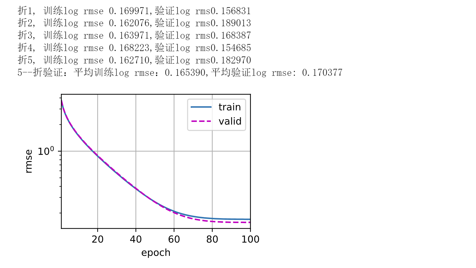
                     legend=['train', 'valid'], yscale='log')
        print(f'折{i + 1}, 训练log rmse {float(train_ls[-1]):f},'
              f'验证log rms{float(valid_ls[-1]):f}')
    return train_l_sum / k, valid_l_sum / k

6. 训练并选择模型

k, num_epochs, lr, weight_decay, batch_size = 5, 100, 5, 0, 64
train_l, valid_l = k_fold(k, train_features, train_labels, 
                          num_epochs, lr, weight_decay, batch_size)
print(f'{k}--折验证：平均训练log rmse：{float(train_l):f},'
      f'平均验证log rmse: {float(valid_l):f}')

7. 提交Kaggle预测

def train_and_pred(train_features, test_featrue, train_labels, test_data,
                   num_epochs, lr, weight_decay, batch_size):
    net = get_net()
    train_ls, _ = train(net, train_features, train_labels, None, None,
                        num_epochs, lr, weight_decay, batch_size)
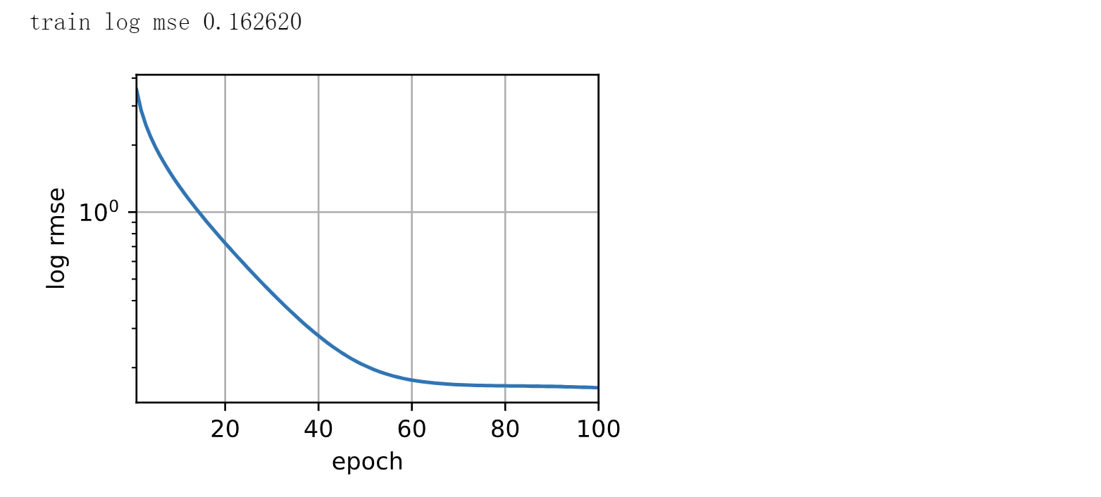
    d2l.plot(np.arange(1, num_epochs + 1), [train_ls], xlabel='epoch',
             ylabel='log rmse', xlim=[1, num_epochs], yscale='log')
    print(f'train log mse {float(train_ls[-1]):f}')
    preds = net(test_featrue).detach().numpy()
    test_data['SalePrice'] = pd.Series(preds.reshape(1, -1)[0])
    submission = pd.concat([test_data['Id'], test_data['SalePrice']], axis=1)
    submission.to_csv('submission.csv', index=False)

train_and_pred(train_features, test_features, train_labels, test_data,
               num_epochs, lr, weight_decay, batch_size)