一.从零开始实现

1.构造线性数据集

import random
import torch
from d2l import torch as d2l

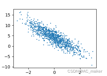
# 根据带有噪声的线性模型构造一个人造数据集。 我们使用线性模型参数w = [2,-3.4].T,b=4.2和噪声项e生成数据集及其标签


def synthetic_data(w, b, num_examples):
    x = torch.normal(0, 1, (num_examples, len(w)))  # 均值为0，方差为1的随机数,n个样本，列数是w的长度
    y = torch.matmul(x, w) + b
    y += torch.normal(0, 0.01, y.shape)  # 均值为0,方差为0.01，形状和y长度一样的噪音
    return x, y.reshape(-1, 1)  # 列向量返回 -1表示行数由pytorch判断,1表示1列


true_w = torch.tensor([2, -3.4])
true_b = 4.2
features, labels = synthetic_data(true_w, true_b, 1000)
# features中的每一行都包含一个二维数据样本，labels中的每一行都包含一维标签值(一个标量)
print('features:', features[0], '\nlabel:', labels[0])
d2l.set_figsize()
d2l.plt.scatter(features[:, 1].detach().numpy(), labels.detach().numpy(), 1)
d2l.plt.show()

运行上述代码随机产生样本和对应图像,如下

 

 对应输出

features: tensor([0.0057, 0.1321]) 
label: tensor([3.7614])

2.生成小批量

def data_iter(batch_size, feature, label):
    num_examples = len(feature)
    indices = list(range(num_examples))
    # 这些样本是随机读取的，没有特定的顺序
    random.shuffle(indices)  # 打乱下标
    for i in range(0, num_examples, batch_size):
        batch_indices = torch.tensor(indices[i:min(i + batch_size, num_examples)])
        # 返回形式features[torch.tensor([371, 275, 458, 585, 506, 961,  96, 606, 790, 468])]
        yield feature[batch_indices], label[batch_indices]  


batch_size = 10
for x, y in data_iter(batch_size, features, labels):
    print(x, '\n', y)
    break

输出 

tensor([[-1.0282,  0.2672],
        [-1.7735, -1.1364],
        [ 0.0604,  0.0238],
        [-0.5580,  0.8345],
        [-2.7177, -1.1851],
        [-3.1734, -0.8336],
        [-0.4015, -1.6372],
        [-0.4167, -0.7885],
        [-0.1123, -0.3314],
        [ 1.2128, -0.2061]]) 

 tensor([[1.2239],
        [4.5136],
        [4.2542],
        [0.2611],
        [2.7865],
        [0.6933],
        [8.9344],
        [6.0326],
        [5.0944],
        [7.3270]])

3.定义初始化模型参数

# 定义初始化模型参数
w = torch.normal(0, 0.01, size=(2, 1), requires_grad=True)  # 均值为0，方差为0.01，2*1矩阵
b = torch.zeros(1, requires_grad=True)
print(b)

输出 

tensor([0.], requires_grad=True)

4.定义模型

def linreg(x, w, b):
    return torch.matmul(x, w) + b

5.定义损失函数-均方损失

def squared_loss(y_hat, y):
    return (y_hat - y.reshape(y_hat.shape))**2 / 2  # 统一格式

6.定义优化算法

def sgd(params, lr, batch_size):
    with torch.no_grad():
        for param in params:
            param -= lr * param.grad / batch_size
            param.grad.zero_()

7.训练过程

lr = 0.03
num_epochs = 3
net = linreg
loss = squared_loss

for epoch in range(num_epochs):
    for x, y in data_iter(batch_size, features, labels):
        l = loss(net(x, w, b), y)  # x 和 y 的小批量损失
        l.sum().backward()
        sgd([w, b], lr, batch_size)  # 使用参数的梯度更新
    with torch.no_grad():
        train_l = loss(net(features, w, b), labels)
        print(f'epoch {epoch + 1}, loss {float(train_l.mean())}')

8.比较真实参数和通过训练学到的参数评估训练成功程度

# 比较真实参数和通过训练学到的参数来评估训练的成功程度
print(f'w的估计误差: {true_w-w.reshape(true_w.shape)}')
print(f'b的估计误差:{true_b-b}')

整体代码浏览

import random
import torch
from d2l import torch as d2l

# 根据带有噪声的线性模型构造一个人造数据集。 我们使用线性模型参数w = [2,-3.4].T,b=4.2和噪声项e生成数据集及其标签


def synthetic_data(w, b, num_examples):
    x = torch.normal(0, 1, (num_examples, len(w)))  # 均值为0，方差为1的随机数,n个样本，列数是w的长度
    y = torch.matmul(x, w) + b
    y += torch.normal(0, 0.01, y.shape)  # 均值为0,方差为0.01，形状和y长度一样的噪音
    return x, y.reshape(-1, 1)  # 列向量返回 -1表示行数由pytorch判断,1表示1列


true_w = torch.tensor([2, -3.4])
true_b = 4.2
features, labels = synthetic_data(true_w, true_b, 1000)
# features中的每一行都包含一个二维数据样本，labels中的每一行都包含一维标签值(一个标量)
print('features:', features[0], '\nlabel:', labels[0])
d2l.set_figsize()
d2l.plt.scatter(features[:, 1].detach().numpy(), labels.detach().numpy(), 1)
d2l.plt.show()

# 定义一个data_iter函数, 该函数接收批量大小,特征矩阵和标签向量作为输入,生成大小为batch_size的小批量


def data_iter(batch_size, feature, label):
    num_examples = len(feature)
    indices = list(range(num_examples))
    # 这些样本是随机读取的，没有特定的顺序
    random.shuffle(indices)  # 打乱下标
    for i in range(0, num_examples, batch_size):
        batch_indices = torch.tensor(indices[i:min(i + batch_size, num_examples)])
        # 返回形式features[torch.tensor([371, 275, 458, 585, 506, 961,  96, 606, 790, 468])]
        yield feature[batch_indices], label[batch_indices]


batch_size = 10
for x, y in data_iter(batch_size, features, labels):
    print(x, '\n', y)
    break


# 定义初始化模型参数
w = torch.normal(0, 0.01, size=(2, 1), requires_grad=True)  # 均值为0，方差为0.01，2*1矩阵
b = torch.zeros(1, requires_grad=True)
print(b)


# 定义模型
def linreg(x, w, b):
    return torch.matmul(x, w) + b


# 定义损失函数
# 均方损失
def squared_loss(y_hat, y):
    return (y_hat - y.reshape(y_hat.shape))**2 / 2  # 统一格式


# 定义优化算法
def sgd(params, lr, batch_size):
    with torch.no_grad():
        for param in params:
            param -= lr * param.grad / batch_size
            param.grad.zero_()


# 训练过程
lr = 0.03
num_epochs = 3
net = linreg
loss = squared_loss

for epoch in range(num_epochs):
    for x, y in data_iter(batch_size, features, labels):
        l = loss(net(x, w, b), y)  # x 和 y 的小批量损失
        l.sum().backward()
        sgd([w, b], lr, batch_size)  # 使用参数的梯度更新
    with torch.no_grad():
        train_l = loss(net(features, w, b), labels)
        print(f'epoch {epoch + 1}, loss {float(train_l.mean())}')

# 比较真实参数和通过训练学到的参数来评估训练的成功程度
print(f'w的估计误差: {true_w-w.reshape(true_w.shape)}')
print(f'b的估计误差:{true_b-b}')

二.简单实现

1.所使用的包

# 通过使用深度学习框架来简洁地实现线性回归模型生成数据集
import numpy as np
import torch
from torch.utils import data
from d2l import torch as d2l
from torch import nn

2.生成数据集

true_w = torch.tensor([2, -3.4])
true_b = 4.2
features, labels = d2l.synthetic_data(true_w, true_b, 1000)

3.构造Pytorch数据迭代器

# 构造一个Pytorch数据迭代器
def load_array(data_arrays, batch_size, is_train=True):
    dataset = data.TensorDataset(*data_arrays)
    return data.DataLoader(dataset, batch_size, shuffle=is_train)


batch_size = 10
data_iter = load_array((features, labels), batch_size)
print(next(iter(data_iter)))

输出

[tensor([[ 0.1219,  1.5637],
        [-0.1459,  0.0461],
        [ 0.3757,  1.1786],
        [ 0.7091, -1.2830],
        [-0.1761,  0.4595],
        [-0.6001,  0.3908],
        [ 0.0719,  0.1164],
        [-1.2292,  0.1371],
        [ 0.4230, -1.6871],
        [-2.2008,  0.8052]]), tensor([[-0.8791],
        [ 3.7520],
        [ 0.9499],
        [ 9.9885],
        [ 2.2831],
        [ 1.6512],
        [ 3.9626],
        [ 1.2727],
        [10.7992],
        [-2.9386]])]

4.使用框架的预定义好的层

# 使用框架的预定义好的层
net = nn.Sequential(nn.Linear(2, 1))  # 输入的维度2，输出的维度是1

5.初始化参数模型

# 初始化模型参数
net[0].weight.data.normal_(0, 0.01)
net[0].bias.data.fill_(0)

6.均方误差

# 计算均方误差使用的是MSELoss类，也称为平方L2范数
loss = nn.MSELoss()

7.实例化sgd实例

# 实例化SGD实例
trainer = torch.optim.SGD(net.parameters(), lr=0.03)

8.训练过程

num_epochs = 3
for epoch in range(num_epochs):
    for x, y in data_iter:
        l = loss(net(x), y)
        trainer.zero_grad()
        l.backward()
        trainer.step()
    l = loss(net(features), labels)
    print(f'epoch：{epoch + 1}, loss：{l:f}')

输出

epoch：1, loss：0.000281
epoch：2, loss：0.000095
epoch：3, loss：0.000094

整体代码浏览

# 通过使用深度学习框架来简洁地实现线性回归模型生成数据集
import numpy as np
import torch
from torch.utils import data
from d2l import torch as d2l
from torch import nn

true_w = torch.tensor([2, -3.4])
true_b = 4.2
features, labels = d2l.synthetic_data(true_w, true_b, 1000)
# 调用框架中现有的API来读取数据


# 构造一个Pytorch数据迭代器
def load_array(data_arrays, batch_size, is_train=True):
    dataset = data.TensorDataset(*data_arrays)
    return data.DataLoader(dataset, batch_size, shuffle=is_train)


batch_size = 10
data_iter = load_array((features, labels), batch_size)
print(next(iter(data_iter)))

# 使用框架的预定义好的层
net = nn.Sequential(nn.Linear(2, 1))  # 输入的维度2，输出的维度是1
# 初始化模型参数
net[0].weight.data.normal_(0, 0.01)
net[0].bias.data.fill_(0)

# 计算均方误差使用的是MSELoss类，也称为平方L2范数
loss = nn.MSELoss()
# 实例化SGD实例
trainer = torch.optim.SGD(net.parameters(), lr=0.03)

num_epochs = 3
for epoch in range(num_epochs):
    for x, y in data_iter:
        l = loss(net(x), y)
        trainer.zero_grad()
        l.backward()
        trainer.step()
    l = loss(net(features), labels)
    print(f'epoch：{epoch + 1}, loss：{l:f}')