Neural Network is often considered a black-box algorithm. Data visualization can help us better understand the principles of this algorithm. Since standard packages don’t give all details of how the parameters are found, we will code a neural network from scratch. And in order to visualize simply the results, we have chosen a simple dataset.

神经网络通常被认为是黑盒算法。 数据可视化可以帮助我们更好地理解该算法的原理。 由于标准软件包并未提供有关如何找到参数的所有详细信息，因此我们将从头开始编写神经网络代码。 为了简单地显示结果，我们选择了一个简单的数据集。

简单的数据集和神经网络结构 (Simple dataset and neural network structure)

Let’s use this simple dataset with only one feature X.

让我们使用仅具有一个特征X的简单数据集。

import numpy as npX=np.array([[-1.51], [-1.29], [-1.18], [-0.64],
[-0.53], [-0.09], [0.13], [0.35],
[0.89], [1.11], [1.33], [1.44]])y=np.array([[0], [0], [0], [0],
[1], [1], [1], [1],[0], [0], [0], [0]])

X is a single column vector with 12 observations, and y is also a column vector with 12 values that represent the target. We can visualize this dataset.

X是具有12个观测值的单列向量，y也是具有12个代表目标值的列向量。 我们可以可视化此数据集。

import matplotlib.pyplot as plt
plt.scatter(X,y)

For those of you who already know how a neural network works, you should be able to find a simple structure by seeing this graph. In the next part, the activation function will be the sigmoid function.

对于已经知道神经网络如何工作的人，您应该可以通过查看此图来找到简单的结构。 在下一部分中，激活函数将为S型函数。

So the question is: how many layers and neurons do we need in order to build a neural network that would fit the dataset above?

所以问题是： 为了建立适合上面数据集的神经网络，我们需要多少层和神经元？

If we use only one neuron it will be the same thing as doing a Logistic Regression because the activation function is the sigmoid function. And we know that it won’t work because the dataset is not linearly separable, and Simple Logistic Regression doesn’t work with not linearly separable data. So we have to add a hidden layer. Each neuron in the hidden layer will result in a linear decision boundary.

如果我们只使用一个神经元，那将与进行Logistic回归相同，因为激活函数是S形函数。 而且我们知道它不起作用，因为数据集不是线性可分离的，并且简单Logistic回归不适用于线性不可分离的数据。 因此，我们必须添加一个隐藏层。 隐藏层中的每个神经元将导致线性决策边界。

In general, a Logistic Regression creates a hyperplane as a decision boundary. Since here we only have one feature, then this hyperplane is only a dot. Visually, we can see that we would need two dots to separate one class from the other. And their values would be around for one -0.5 and the other 0.5.

通常，逻辑回归会创建一个超平面作为决策边界。 因为这里我们只有一个特征，所以这个超平面只是一个点。 从视觉上看，我们需要两个点来将一个类与另一个类分开。 它们的值大约为-0.5，另一个为0.5。

So a neural network with the following structure would be a good classifier for our dataset.

因此，具有以下结构的神经网络对于我们的数据集将是一个很好的分类器。

If it is not clear for you, you can read this article.

如果您不清楚，则可以阅读本文。

使用scikit学习MLPClassifier (Using scikit learn MLPClassifier)

Before building the neural network from scratch, let’s first use algorithms already built to confirm that such a neural network is suitable, and visualize the results.

在从头开始构建神经网络之前，让我们首先使用已经构建的算法来确认这种神经网络是否合适，并可视化结果。

We can use the MLPClassifier in scikit learn. In the following code, we specify the number of hidden layers and the number of neurons with the argument hidden_layer_sizes.

我们可以在scikit中使用MLPClassifier学习。 在下面的代码中，我们使用参数hidden_​​layer_sizes指定隐藏层的数量和神经元的数量。

from sklearn.neural_network import MLPClassifierclf = MLPClassifier(solver=’lbfgs’,hidden_layer_sizes=(2,), activation=”logistic”,max_iter=1000)clf.fit(X, y)

Then we can calculate the score. (You should get 1.0, otherwise, you may have to run the code again because of local minimums).

然后我们可以计算分数。 (您应该获得1.0，否则，由于局部最小值，您可能不得不再次运行代码)。

clf.score(X,y)

So great, how can we visualize the results of the algorithm? Since we know that this neural network is made by 2+1 Logistic Regression, we can get the parameters with the following code.

太好了，我们如何可视化算法的结果？ 由于我们知道该神经网络是由2 + 1 Logistic回归构成的，因此可以使用以下代码获取参数。

clf.coefs_
clf.intercepts_

How do we interpret the results?

我们如何解释结果？

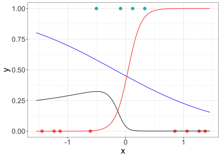
For clf.coefs_, you will get (for example):

对于clf.coefs_ ，您将获得(例如)：

[array([[-20.89123833, -8.09121263]]), array([[-20.19430919], [ 17.74430684]])]

And for clf.intercepts_

对于clf.intercepts_

[array([-12.35004862, 4.62846821]), array([-8.19425129])]

The first items of the lists contain the parameters for the hidden layer, and the second items contain the parameters for the output layer.

列表的第一项包含隐藏层的参数，第二项包含输出层的参数。

With these parameters, we can plot the curves:

使用这些参数，我们可以绘制曲线：

def sigmoid(x):
    return 1.0/(1+ np.exp(-x))plt.scatter(X,y)
a1_1=sigmoid(xseq*clf.coefs_[0][0,0]+clf.intercepts_[0][0])
a1_2=sigmoid(xseq*clf.coefs_[0][0,1]+clf.intercepts_[0][1])
output=sigmoid(a1_1*clf.coefs_[1][0]+a1_2*clf.coefs_[1][1]+clf.intercepts_[1])plt.plot(xseq,a1_1,c=”red”)
plt.plot(xseq,a1_2,c=”blue”)
plt.plot(xseq,output,c=”black”)

And we can get the following graph:

我们可以得到下图：

• The red one is the result of the neuron 1 of the hidden layer
  红色是隐藏层神经元1的结果
• The blue one is the result of the neuron 2 of the hidden layer
  蓝色的是隐藏层的神经元2的结果
• The black one is the output
  黑色的是输出

If you run the code, you may get another result, because the loss function has several global minimums.

如果运行代码，则可能会得到另一个结果，因为损失函数具有多个全局最小值。

In keras, it is of course also possible to create the same structure:

在keras中 ，当然也可以创建相同的结构：

from keras.models import Sequential
from keras.layers import Dense
model = Sequential()
model.add(Dense(2, activation=’sigmoid’))
model.add(Dense(1, activation=’sigmoid’))
model.compile(loss=’binary_crossentropy’, optimizer=’adam’, metrics=[‘accuracy’])
model.fit(X_train, y_train, epochs=300)

从头开始编码 (Coding from scratch)

Now the question is how are all the seven parameters found? One method is to use gradient descent.

现在的问题是如何找到所有七个参数？ 一种方法是使用梯度下降。

正向传播 (Forward propagation)

First, let’s do the forward propagation.

首先，让我们进行正向传播。

For each neuron, we have to find the weight w and the bias b. Let’s try some random values.

对于每个神经元，我们必须找到权重w和偏差b。 让我们尝试一些随机值。

plt.scatter(X,y)
plt.plot(xseq,sigmoid(xseq*(-11)-11),c="red")

Since there are two neurons, we can do a matrice multiplication by creating matrices for the parameters:

由于有两个神经元，我们可以通过为参数创建矩阵来进行矩阵乘法：

• the weight matrix should have two columns. (Since here the input data has one column, then the weight matrix should have one row and two columns). We can do a random initialization, and choose some values.
  权重矩阵应具有两列。 (由于此处输入数据只有一列，所以权重矩阵应该有一行和两列)。 我们可以进行随机初始化，然后选择一些值。
• the bias should have the same structure.
  偏差应具有相同的结构。

w1=np.random.rand(X.shape[1],2) # random initialization
w1=np.array([[-1,9]])
b1=np.array([[-1,5]])z1=np.dot(X, w1)+b1
a1=sigmoid(z1)

If you are just reading and not running a notebook at the same time, one exercise to do is to answer the following questions:

如果您只是在阅读而不同时在运行笔记本，则要做的一项练习是回答以下问题：

• What is the dimension of np.dot(X, w1)?
  np.dot(X，w1)的维数是多少？
• What is the dimension of z1?
  z1的维数是多少？
• Why is it OK to do addition? What if b1 is a simple 1d-array?
  为什么可以加法？ 如果b1是一个简单的一维数组怎么办？
• What is the dimension of a1?
  a1的维数是多少？

If we replace the input X by xseq created before, we can plot the curves:

如果用之前创建的xseq替换输入X，则可以绘制曲线：

a1_seq=sigmoid(np.dot(xseq.reshape(-1,1), w1)+b1)plt.scatter(X,y)
plt.plot(xseq,a1_seq[:,0],c="red")
plt.plot(xseq,a1_seq[:,1],c="blue")

Now for the output, it is a very similar calculation.

现在对于输出，这是一个非常相似的计算。

• The weight matrix has now the rows because the hidden layer results in a matrix of two columns.
  权重矩阵现在具有行，因为隐藏层导致两列矩阵。
• The bias matrix is a scalar
  偏差矩阵是一个标量

w2 = np.random.rand(2,1)
b2=0
output=sigmoid(np.dot(a1,w2)+b2)

Then we can plot the output, with the other curves

然后我们可以绘制输出以及其他曲线

output_seq=sigmoid(np.dot(a1_seq,w2)+b2)plt.scatter(X,y)
plt.plot(xseq,a1_seq[:,0],c=”red”)
plt.plot(xseq,a1_seq[:,1],c=”blue”)
plt.plot(xseq,output_seq,c=”black”)

As you can see, the randomly chosen parameters are not good.

如您所见，随机选择的参数不好。

Just to sum up the forward propagation:

总结一下正向传播：

def feedforward(input,w1,w2,b1,b2):
    a1 = sigmoid(np.dot(input, w1)+b1)
    output = sigmoid(np.dot(a1, w2)+b2)
    return output

成本函数的可视化 (Visualization of the cost function)

The suitable parameters are those which minimize the cost function. We can use the cross-entropy:

合适的参数是那些使成本函数最小的参数。 我们可以使用交叉熵：

The function can coded as below:

该函数可以编码如下：

def cost(y,output):
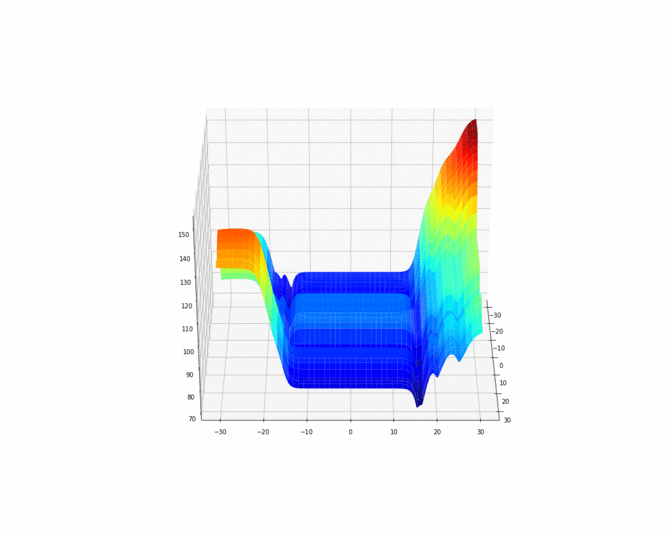
    return -np.sum(y*np.log(output)+(1-y)*np.log(1-output))/12

Since there are 7 parameters, visualizing the cost function is not easy. Let’s just choose one of them to vary. For example the first weight in w1.

由于有7个参数，因此可视化成本函数并不容易。 我们只选择其中之一进行更改。 例如，w1中的第一个权重。

b1=np.array([[16.81,-23.41]])
w2= np.array([28.8,-52.89])
b2=-17.53p = np.linspace(-100,100,10000)for i in range(len(p)):
    w1=np.array([[p[i],-37.94]])
    output=feedforward(X,w1,w2,b1,b2)
    cost_seq[i]=cost(y,output)

And you can see that it is not convex at all.

您会看到它根本不是凸的。

And it is also possible to vary two parameters.

并且还可以改变两个参数。

In order to better visualize the cost function, we can also make an animation.

为了更好地可视化成本函数，我们还可以制作动画。

Now let find some suitable global minimums of this cost function using gradient descent which is call backpropagation.

现在，使用梯度下降(称为反向传播)找到此成本函数的一些合适的全局最小值。

反向传播 (Backpropagation)

Partial derivatives can be ugly, but fortunately, with the cross-entropy as a loss function, there are some simplifications in the final results.

偏导数可能很难看，但是幸运的是，由于交叉熵是一种损失函数，最终结果有一些简化。

Here is the cost function again:

这又是成本函数：

• Please note that when you use the cost function to calculate the cost of a model, then the input variables for this function are the output of the model and the real value of the target variable.
  请注意，当您使用cost函数计算模型的成本时，此函数的输入变量是模型的输出和目标变量的实际值。
• If we try to find the optimum parameters of the model, then we consider that the input variables for this cost function are these parameters. And we are going to calculate the partial derivatives of the cost function with respect to every parameter.
  如果我们试图找到模型的最佳参数，那么我们认为该成本函数的输入变量就是这些参数。 而且，我们将针对每个参数计算成本函数的偏导数。

For the partial derivative with respect to w1, using the chain rule, we have:

对于使用链规则的关于w1的偏导数，我们有：

First, for the sigmoid function, the derivative can be written as:

首先，对于S形函数，导数可写为：

(Please note that the cost function is a sum of functions, and the partial derivative of a sum of functions is the sum the partial derivates of the functions, so in order to simplify the notation, we will drop the sum symbol, or to be exact, the mean calculation).

(请注意，代价函数是函数的和，函数和的偏导数是函数的偏导数之和，因此，为了简化表示法，我们将求和符号删除，或者将精确，均值计算)。

Let’s first calculate the first two items as below:

让我们首先计算如下两个项目：

And we can notice that they can be simplified to (yhat-y).

我们可以注意到，它们可以简化为(yhat-y)。

Then we have the final result for the w1:

然后我们得到了w1的最终结果：

For b1, the expression is quite similar, as the only difference is the last partial derivative:

对于b1，表达式非常相似，因为唯一的不同是最后的偏导数：

We are going to code the computation with matrix multiplication. Before coding, we can ask ourselves some questions (and answer them):

我们将使用矩阵乘法对计算进行编码。 在编码之前，我们可以问自己一些问题(并回答)：

• What is the dimension of the residuals (yhat — y)? It is a column vector and the number of rows is equal to the number of total observations.
  残差的维数(yhat-y)是多少？ 它是列向量，行数等于总观测数。
• What is the dimension of w2? It is a matrix of two rows and one column. Remember, it is the weight matrix for the two hidden neurons, to compute the output.
  w2的维数是多少？ 它是两行一列的矩阵。 请记住，它是两个隐藏神经元的权重矩阵，用于计算输出。
• What is the dimension of (yhat — y)*w2? Since the dimension w2 is (2,1), we can not do a simple multiplication. What should we do? We can transpose the w1 matrix. Then (yhat — y)*w2 will give us a matrix of two columns and 12 observations. It is perfect because we want to do the computation for each of the weights.
  (yhat-y)* w2的维数是多少？ 由于维数w2为(2,1)，因此我们无法进行简单的乘法运算。 我们应该做什么？ 我们可以转置w1矩阵。 然后(yhat-y)* w2将给我们一个包含两列和12个观察值的矩阵。 这是完美的，因为我们想对每个权重进行计算。
• What is the dimension of a1? It is the results of the hidden layer. Since we have two neurons, a1 has two columns and 12 observations. And the multiplication with the previous matrix will be element-wise multiplication.
  a1的维数是多少？ 这是隐藏层的结果。 由于我们有两个神经元，所以a1有两列和12个观察值。 与先前矩阵的乘法将是逐元素乘法。
• All this is very consistent because, in the end, we will get a matrix of 2 columns and 12 observations. And the first column is associated with the weight of the first neuron, and the second column is associated with the weight of the second neuron in the hidden layer.
  所有这些都是非常一致的，因为最终，我们将获得一个由2列和12个观察值组成的矩阵。 第一列与第一神经元的权重相关联，第二列与隐藏层中第二神经元的权重相关联。

Let’s do some coding:

让我们做一些编码：

d_b1_v=np.dot((output-y), w2.T) * a1*(1-a1)

What does this matrix represent? We can show the partial derivative with respect to b1 again.

这个矩阵代表什么？ 我们可以再次显示关于b1的偏导数。

The matrix d_b1_v is the partial derivative for all observations. And to get the final derivatives, we have to calculate the sum of those associated with all observations (remember, L is a sum of functions), and calculate the average value.

矩阵d_b1_v是所有观测值的偏导数。 为了获得最终的导数，我们必须计算与所有观测值相关的和(请记住，L是函数的总和)，并计算平均值。

d_b1=np.mean(d_b1_v,axis=0)

For w1, we have to take x into account. For each observation, we have to multiply the value obtained by previous partial derivatives by the value of x, then sum them all. This is exactly a dot product. And to obtain the average value, we have to divide by the number of observations.

对于w1，我们必须考虑x。 对于每个观察，我们必须将先前的偏导数获得的值乘以x的值，然后将它们全部求和。 这正是一个点积。 为了获得平均值，我们必须除以观察次数。

d_w1 = np.dot(X.T, d_b1_v)/12

Now, let continue for the parameters of the output layer. It will be much easier.

现在，让我们继续输入输出层的参数。 这样会容易得多。

We already have:

我们已经有：

So the derivatives with respect to w2 and b2 are:

因此，关于w2和b2的导数为：

For b2, we just have to sum the residuals

对于b2，我们只需要对残差求和

np.sum(output-y)/12

For w2, it is the dot product between a1 (results of layer 1) and the residuals.

对于w2，它是a1(第1层的结果)和残差之间的点积。

np.dot(a1.T, (output-y))/12

包装中的最终算法 (Final algorithm in a wrap)

Now we can create a class to include the two steps of forward propagation and backward propagation.

现在我们可以创建一个类，以包括正向传播和反向传播两个步骤。

I used the python code based on this very popular article. You may already have read it. The differences are

我根据这篇非常受欢迎的文章使用了python代码。 您可能已经阅读过。 区别是

• the loss function (cross-entropy instead of MSE)
  损失函数(交叉熵而不是MSE)
• adding a learning rate
  增加学习率

class NeuralNetwork:
    def __init__(self, x, y):
        self.input = x
        self.w1 = np.random.rand(self.input.shape[1],2)
        self.w2 = np.random.rand(2,1)
        self.b1 = np.zeros(2)
        self.b2 = 0.0
        self.y = y
        self.output = np.zeros(self.y.shape)    def feedforward(self):
        self.a1 = sigmoid(np.dot(self.input, self.w1)+self.b1)
        self.output = sigmoid(np.dot(self.a1, self.w2)+self.b2)    def backprop(self):
        lr=0.1        res=self.output-self.y        d_w2 = np.dot(self.a1.T, res)
        d_b2 = np.sum(res)
        d_b1_v=np.dot(res, self.w2.T) * self.a1*(1-self.a1)
        d_b1 = np.sum(d_b1_v,axis=0)
        d_w1 = np.dot(self.input.T, d_b1_v)        self.w1 -= d_w1*lr
        self.w2 -= d_w2*lr
        self.b1 -= d_b1*lr
        self.b2 -= d_b2*lr

It is then possible to store the intermediate values of the 7 parameters during the gradient descent and plot the curves.

然后可以在梯度下降过程中存储7个参数的中间值并绘制曲线。

The animation is made with graphs from R code. So if you are interested in R code of the neural network from scratch, please comment.

动画是使用R代码中的图形制作的。 因此，如果您从头开始对神经网络的R代码感兴趣，请发表评论。

If you the code is difficult for you to understand, I also created an Excel (Google Sheet) file to do the gradient descent. If you are interested, please let me know in the comments. Yes, you may think that is it crazy to do machine learning in Excel, and I agree with you, especially after having done all the steps of gradient descent for all the seven parameters. But the objective is to better understand. And for that, Excel is an excellent tool.

如果您的代码难以理解，我还创建了一个Excel(Google表格)文件来进行梯度下降。 如果您有兴趣，请在评论中让我知道。 是的，您可能会认为在Excel中进行机器学习非常疯狂，并且我也同意您的观点，尤其是在对所有七个参数都完成了梯度下降的所有步骤之后。 但目的是更好地理解。 因此，Excel是一个出色的工具。