图神经网络与分子表征：8. TFN

兴致冲冲的我抱着 2023-ICML-eSCN 看了好几天，毫无头绪，因为 2023-ICML-eSCN 是建立在 NequIP 这类多通道模型的基础之上的。在进一步挖掘后，我发现这些论文里频繁提到老文献 TFN，以及其背后的 Python 库 e3nn.

frank_haha

2290人浏览 · 2024-07-01 01:13:01

frank_haha · 2024-07-01 01:13:01 发布

最近在读前沿论文时，发现很多人开始提及 SO2 关键词。简单梳理发展路线是：2023-ICML-eSCN 首次提出 SO2, 次年 ICLR 含有 SO2 模块的 2024_ICLR_EquiformerV2 就见刊了。预测哈密顿量方面 DeepH 的正统续作 DeepH2 也采用了 SO2 模块。

是什么原因让 SO2 模块这么受欢迎呢？上述几篇论文频繁提及的是，使用 SO2 能够大幅降低 tensor product 的计算量，使得模型能够拓展到更高的 degree 上。换言之，以前的这些模型本身也可以使用更高 degree 的张量，但计算量不允许，使用 SO2 就可以了，精度提高同时，速度还能受控制。

在学习 SO2（也就是 2023-ICML-eSCN 这篇论文）的过程中，我发现，原文里提到的很多概念很难理解。这是因为，我在这一领域的学习是按照本系列的撰写路线来的。从 SchNet 到 DimeNet, PaiNN, LEFTNet，这些模型最多只用了标量+向量双通道，而使用更高维通道的模型，本人涉猎尚浅，一直以“速度慢，精度也没见有多高”这种理由回避。例如，NequIP, Allegro, SEGNN 这种优秀模型。

当时我对这些模型的理解如下图所示：

请添加图片描述

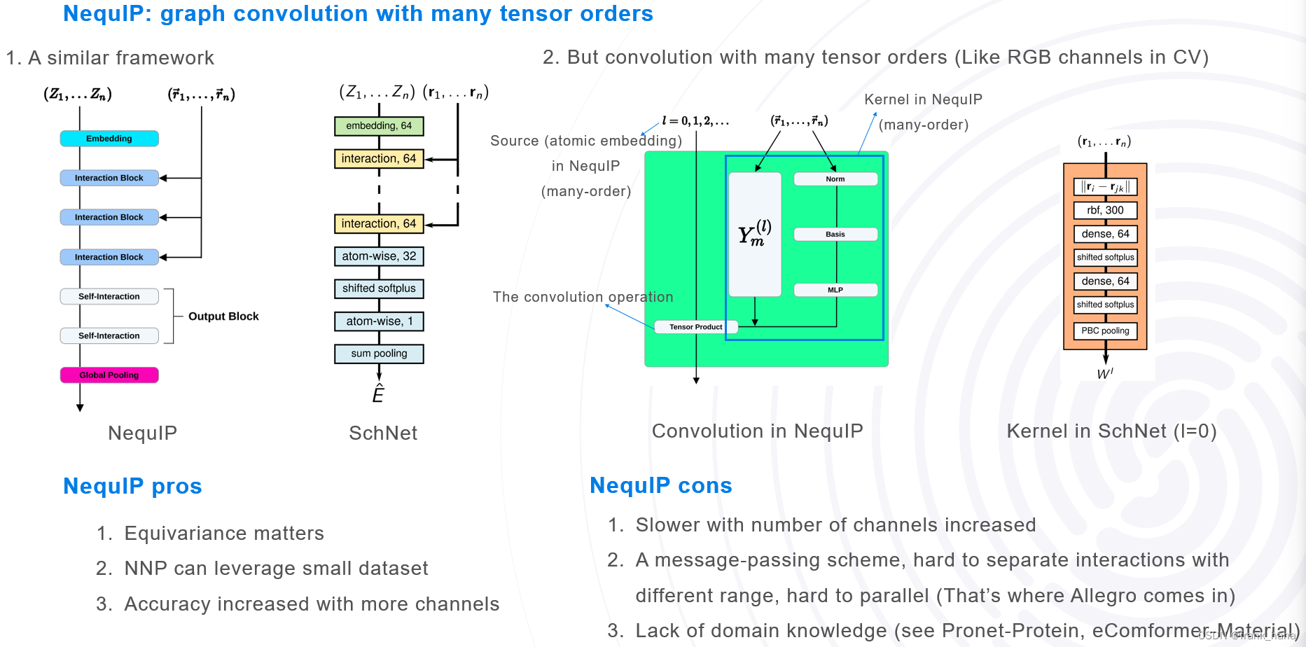
拿 NequIP 和 SchNet 做对比，二者的主框图是基本一致的，都是图卷积的模式。唯一区别在于 NequIP 在对原子做内嵌时增加了通道数，从原来的标量通道，增加到可调节的高维通道：l = 1 就是标量+向量，l = 2 是标量+向量+二维张量（矩阵）。就类似 CV 中的卷积，从只能处理灰白图像的单通道，拓展到了能处理彩色图像的 RGB 三通道。通道数越多，精度越高，速度越慢。这些都很好理解。

但是作者具体是怎么实现的，当时没有深究，于是就出现了开头讲到的困境：因为回避一些技术发展路线，而无法跟上当前领域最新进展。

TFN 的第一次面世已经是 2018 年了，比 NequIP 早 3 年，但二者的框架基本一致。是 TFN 奠定了上述多通道模型的技术路线，首次给出了张量积，球谐函数，CGC 系数等概念，追封为开山之作不为过。

e3nn 是多通道模型均采用的表征高维张量的 Python 库。大家可以在类 NequIP 模型（以 Genome 为例）中看到直接引入 e3nn 的字段。

from .e3nn_layer import FullyConnectedTensorProductE3nn

为了学习 e3nn，我又开始全网寻找教程，最终发现 Github 上一个教程：thu-wangz17/e3nn_notes: e3nn从入门到放弃 (github.com)

教程里简明扼要的对 e3nn 涉及的主要概念进行了讲解。此处，我按照自己的理解对相关概念进行拓展。（非常白话可能有不严谨的地方）（以及 e3x 也是很棒的教材）

首先，什么是群？

群是包含群元的集合，有以下几个性质：

请添加图片描述

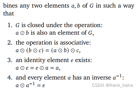
就是闭包性、交互性等等，这些性质后面基本是不会用到。

有群就有群元，我们以常用群 SO3 为例，SO3 的群元，如果用矩阵形式表示的话，是一个 3x3 的矩阵。注意，并不是所有的 3x3 的矩阵都是 SO3 的群元，此处的 3x3 的矩阵指，任何一个 nx3 的矩阵乘以该 3x3 矩阵相当于在空间中进行了旋转，如下图所示：

请添加图片描述

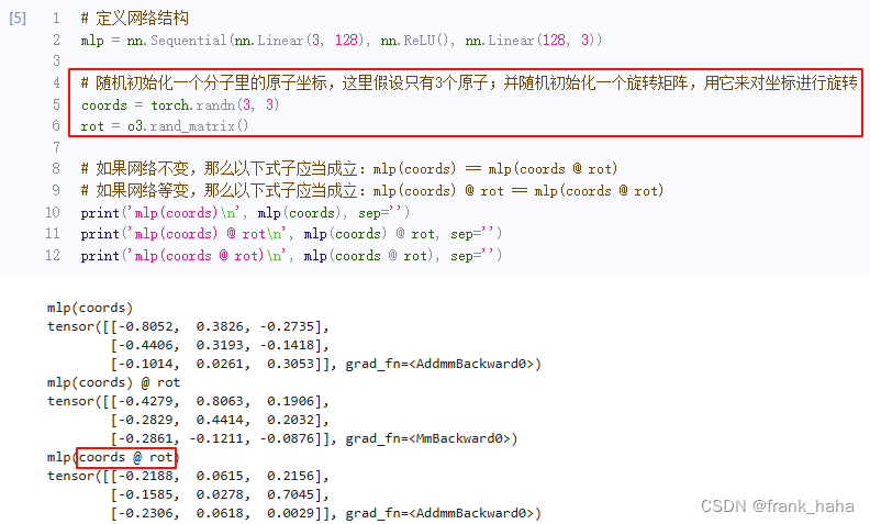
也就是说，所有满足“相乘即旋转”性质的矩阵的几何构成了 SO3 群， SO3 群的群元可以用 3x3 的矩阵表示。

更近一步

在数学里，大家十分崇尚简约又有秩序的美。例如，在高中数学里，我们学过：任何向量可以由单位向量及其系数表示。比如，我们常说的 xy 坐标系下的坐标 (a, b)，其实就是 a*单位x向量+b*单位y向量。

在群论中，我们认为，任何群元可以由一组不可约基组表示，形成类似基组*系数的组合，我们将其称为不可约表示 (irreducible representations, irreps)。我们认为随机抽取的群元是高维向量空间中的一点。

e3nn.o3.Irreps('10x0e + 5x1o + 2x2e')中10x0e表示有 $10$ 个 $l = 0$ 的偶宇称(e)特征，奇宇称为o。标量为 $l = 0$ 的偶宇称特征， $\because 2l+1=1$ ，表明维度为1-dim，并且标量不随宇称变化（不会随宇称改变符号）。矢量为 $l = 1$ 的奇宇称特征。

这句话就是多通道模型中常常看到的，初始化基组的方法。

10x0e：10 个零维（scalar）偶宇称（even）特征
5x1o：5 个 1维（vector）奇宇称（odd）特征
2x2e：2 个 2维（类似二维矩阵）偶宇称特征

下面随机初始化一个群元，并将其转化为不可约表示（又叫 Wigner-D matrix），再进行可视化（下面源自thu-wangz17/e3nn_notes: e3nn从入门到放弃 (github.com)）

import os

os.environ['KMP_DUPLICATE_LIB_OK'] = "True"

import matplotlib.pyplot as plt

import torch
from torch import nn
from e3nn import o3


irreps = o3.Irreps("10x0e + 5x1o + 2x2e")

rot = -o3.rand_matrix()

D = irreps.D_from_matrix(rot)
print(D.size())

plt.imshow(D, cmap='bwr', vmin=-1, vmax=1)

在该例中，我们

irreps = o3.Irreps("10x0e + 5x1o + 2x2e")确定不可约表示
rot = -o3.rand_matrix()产生一个随机旋转矩阵。
- 旋转矩阵
  $\begin{aligned} \mathcal{M}(\alpha, \beta, \gamma) &= \mathcal{R}_z(\alpha)\mathcal{R}_x(\beta)\mathcal{R}_z(\gamma)\\ &= \begin{pmatrix} \cos\alpha\cos\gamma -\cos\beta\sin\alpha\sin\gamma & -\cos\beta\cos\gamma\sin\alpha - \cos\alpha\sin\gamma & \sin\alpha\sin\beta \\ \cos\gamma\sin\alpha + \cos\alpha\cos\beta\sin\gamma & \cos\alpha\cos\beta\cos\gamma - \sin\alpha\sin\gamma & -\cos\alpha\sin\beta \\ \sin\beta\sin\gamma & \cos\gamma\sin\beta & \cos\beta \end{pmatrix} \end{aligned}$
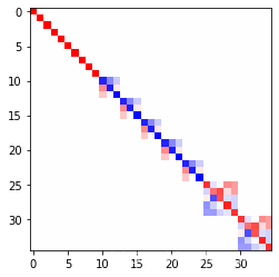
D = irreps.D_from_matrix(rot)是对应于旋转矩阵的表示。由于表示为10x0e + 5x1o + 2x2e，因此结果为10个标量（ $l = 0$ ）、5个 $3\times 3$ 矩阵与2个 $\times 5$ 的矩阵的直和。
- 直和得到的为对角块矩阵。
- D.size()为 $(35, 35)$ ，其中 $35 = 10 * (2 * 0 + 1) + 5 * (2 * 1 + 1) + 2 * (2 * 2 + 1)$ 。

如下图所示：

请添加图片描述

最后，我们看一下 TFN 中的实现：

$f_i^\prime = \frac{1}{\sqrt{z}} \sum_{\mathcal{N}_i}f_j\otimes h(\parallel \vec{x}_{ij}\parallel)Y(\frac{\vec{x_{ij}}}{\parallel \vec{x}_{ij}\parallel})$

其中 $f_j$ 和 $f_i^\prime$ 分别为节点 $j$ 的特征和节点 $i$ 在下一神经网络层的特征， $z$ 为节点 $i$ 的度, $\mathcal{N}*_i$ 为节点 $i$ 的近邻， $\vec{x}_{ij}$ 为节点 $i$ 和 $j$ 之间的相对矢量。 $h$ 为MLP， $Y$ 为球谐函数。 $x\otimes (w)y$ 为 $x$ 和 $y$ 的直积，其中参数为 $w$ ，对应TFN的 $h(\cdot)$ 。

from torch_cluster import radius_graph
from torch_scatter import scatter
from e3nn import nn as enn
from e3nn.math import soft_one_hot_linspace


irreps_input = o3.Irreps("10x0e + 10x1e")
irreps_output = o3.Irreps("20x0e + 10x1e")

num_nodes = 100
pos = torch.randn(num_nodes, 3)  # random node positions

# create edges
max_radius = 1.8
edge_src, edge_dst = radius_graph(pos, max_radius, max_num_neighbors=num_nodes - 1)

edge_vec = pos[edge_dst] - pos[edge_src]

# compute z
num_neighbors = len(edge_src) / num_nodes

f_in = irreps_input.randn(num_nodes, -1)
print(f_in.size())

irreps_sh = o3.Irreps.spherical_harmonics(lmax=2)
print(irreps_sh)

sh = o3.spherical_harmonics(irreps_sh, edge_vec, normalize=True, normalization='component')
print(edge_vec.size(), sh.size())

* f_in为 $(100, 40)$ 的张量，其中100为节点数num_nodes， $40 = 10 * (2 * 0 + 1) + 10 * (2 * 1 + 1)$ 。

* o3.Irreps.spherical_harmonics(lmax=2)表示取球谐函数到 $l$ 最大为2，即取 $0, 1, 2$ 。

* sh的第一个维度为edge_src的维度，即边的个数；第二个维度 $= (2 * 0 + 1) + (2 * 1 + 1) + (2 * 2 + 1)$ 。

tp = o3.FullyConnectedTensorProduct(irreps_in1=irreps_input, irreps_in2=irreps_sh, irreps_out=irreps_output, shared_weights=False)

print(tp)
print(tp.instructions)
print(o3.FullTensorProduct(irreps_in1=irreps_input, irreps_in2=irreps_sh))

* tp计算了 $f_j \otimes (w) Y(\cdot)$ ，其中irreps_input对应着节点 $j$ 的特征的表示，irreps_sh对应着球谐函数 $Y$ 。 $f_i^\prime$ ，即输出的维度由irreps_out控制。

* o3.FullyConnectedTensorProduct实际上是双线性计算，权重的维度为(output, $input_1$ , $input_2$ )。在上面的例子中，irreps_inputs ( $input_1$ )为10x0e+10x1e，球谐函数irreps_sh ( $input_2$ )为1x0e+1x1o+1x2e。暂时先不考虑输出的表示要求，正常的张量积(o3.FullyTensorProduct)将会得到

(10 × 0e + 10 × 1e) ⊗ (1 × 0e + 1 × 1o + 1 × 2e) 
= 10 × 0e ⊗ 1 × 0e + 10 × 1e ⊗ 1 × 0e + 10 × 0e ⊗ 1 × 1o + 10 × 1e ⊗ 1 × 1o + 10 × 0e ⊗ 1 × 2e + 10 × 1e ⊗ 1 × 2e
= 10 × 0e + 10 × 1e + 10 × 10 + 10 × (0 ⊕ 1 ⊕ 2)o + 10 × 2e + 10 × (1 ⊕ 2 ⊕ 3)e
= 10 × 0o + 10 × 0e + 20 × 1o + 20 × 1e + 10 × 2o + 20 × 3e

推导中利用了 $e\times e=e, e\times o=o, l_1\otimes l_2=\bigoplus_{l_i=\vert l_1-l_2\vert}^{l_1+l_2}l_i$ 。而对于o3.FullyConnectedTensorProduct相当于只取正常的张量积中对应的部分，并令这部分前的权重为可学习的参数，如果irreps_output中包含不在正常的张量积中的项，则其对应的权重数量为0 (e.g. o3.FullyConnectedTensorProduct(o3.Irreps('10x0e'), o3.Irreps('3x1o'), o3.Irreps('4x0o'))输出为FullyConnectedTensorProduct(10x0e x 3x1o -> 4x0o | 0 paths | 0 weights)，因为 $l_1=0$ 的偶宇称与 $l_2=1$ 的奇宇称的输出只能为 $l = 1$ 的奇宇称，可以验证o3.FullyConnectedTensorProduct(o3.Irreps('10x0e'), o3.Irreps('3x1o'), o3.Irreps('4x1o'))的输出为FullyConnectedTensorProduct(10x0e x 3x1o -> 4x1o | 120 paths | 120 weights)，存在可学习权重)。

* o3.FullyConnectedTensorProduct的权重数量计算：

e.g. 以上面的cell中的输入和输出为例，输入为10x0e + 10x1e和1x0e+1x1o+1x2e，输出为20x0e + 10x1e。其中输出为 $20\times 0e$ 的输入部分只能为 $10\times 0e \otimes 1\times 0e$ ，对应的权重数量为 $20\times 10 \times 1=200$ (双线性计算的权重维度)，而 $10\times 1e$ 的输入部分只能为 $10\times 1e \otimes 1\times 0e + 10\times 1e \otimes 1\times 2e$ ，对应的权重数量为 $10\times 10 \times 1 + 10 \times 10 \times 1=200$ ，所以总的权重数量为400 (可通过tp.instructions查看，显示的path_shape即为这几个路径对应的权重的维度)。

num_basis = 10

edge_length_embedding = soft_one_hot_linspace(
    edge_vec.norm(dim=1),
    start=0.0,
    end=max_radius,
    number=num_basis,
    basis='smooth_finite',
    cutoff=True,
)
edge_length_embedding = edge_length_embedding.mul(num_basis**0.5)

print(edge_vec.size(), edge_length_embedding.size())

fc = enn.FullyConnectedNet([num_basis, 16, tp.weight_numel], torch.relu)
weight = fc(edge_length_embedding)

print(weight.shape)

print('\nParameters of network h:')
for i in fc.parameters():
    print(i.size())

summand = tp(f_in[edge_src], sh, weight)

print('\n', summand.size())

* soft_one_hot_linspace将每个x值根据选取的基组投影 $\frac{1}{Z}f_i(x)$ 。

* 上述操作是为了构建 $h(\parallel \vec{x_{ij}} \parallel)$ ： $h(\cdot)$ 将原子间距映射为双线性计算中张量积的系数。为了构建该系数，首先利用原子间距产生维度为(边的个数, 基组数量)的特征作为网络的输入。

* o3.nn.FullyConnectedNet接受一个列表作为参数，类似于torch.nn.Sequential构建一个多层神经网络网络。网络的输入维度应等于基组的数量，输出应等于tp的所需的权重的维度。

* tp(f_in[edge_src], sh, weight)计算了 $x\otimes (w)y$ 。

f_out = scatter(summand, edge_dst, dim=0, dim_size=num_nodes).div(num_neighbors ** 0.5)

print(f_out.size())

在这里插入图片描述

torch_scatter.scatter第一个参数为输入的特征，第二个参数为指标，以一维张量为例，scatter函数将根据指标将相同的指标所对应的输入特征进行约化聚合。因此f_out是根据edge_dst将相同指标的summand聚合 (相同指标的edge_dst代表着对应的edge_src指向相同的目标节点，因此这些源节点为该目标节点 $i$ 的近邻 $\mathcal{N}_i$ )。
.div(num_neighbors ** 0.5)计算了 $\frac{1}{\sqrt{z}}$ 。