本人处于学习摸索阶段，文中错误难免，欢迎指正。

       数据预测整体思路：

       本文使用LogisticRegression建模对信贷业务进行违约预测，考虑该模型对变量的要求主要有：

       1.变量之间不应存在较强的线性相关性和多重共线性

       2.变量具有显著性：变量对应的系数P值，P值越小越好

       3.变量具有合理的业务含义，符合风控逻辑：从系数的符号判定

       4.缺失值和异常值对变量的影响较大

       基于以上要求，对数据进行梳理，具体做法如下：

     （一）数据预处理

       1.了解数据自带的字典解释，查看数据整体特征，删除没有业务含义的变量。

       2.分离数值型变量和类别型变量，部分数值型变量存在输入不规范问题

       3.使用sql处理不规范输入问题

       4.使用箱线图查看数值型变量分布的合理性，处理异常值

     （二）数据相关性分析

       1.线性相关性分析，使用pearson计算相关系数，相关性大于0.6的特征，使用pearsonr查看p值。

       2.使用逐步回归法（stepwise regression）查看特征之间的共线性，筛选并删除具有多重共线性的变量，本文使用这种方法对特征做筛选。

     （三） 变量分箱，woe编码，iv值计算

       1.变量分箱：特征分箱也是连续特征离散化，将连续性的特征进行分段，使其变成一个个离散的区间，离散化的特征对异常值有很强的鲁棒性，降低了模型过拟合的风险。首先根据woe的单调性查看合适的分箱区间，确定好分箱区间，对变量进行分箱、编码、计算iv值。

       2.根据特征iv值，再一次筛选特征。

       （四）模型训练，评估模型效果

       1.模型划分为训练集和测试集

       2.使用AUC和KS对模型效果进行评估

一、数据整体情况

1.数据读取：共有28个特征，100000行 ，同一个客户有多条业务记录，预测每一条记录违约情况

import  pandas as pd
import numpy as np
data = pd.read_csv(r"D:\new_job\KAGGLE\kaggle\train.csv")
print(data.columns)
print(data.shape)

Index(['ID', 'Customer_ID', 'Month', 'Name', 'Age', 'SSN', 'Occupation',
       'Annual_Income', 'Monthly_Inhand_Salary', 'Num_Bank_Accounts',
       'Num_Credit_Card', 'Interest_Rate', 'Num_of_Loan', 'Type_of_Loan',
       'Delay_from_due_date', 'Num_of_Delayed_Payment', 'Changed_Credit_Limit',
       'Num_Credit_Inquiries', 'Credit_Mix', 'Outstanding_Debt',
       'Credit_Utilization_Ratio', 'Credit_History_Age',
       'Payment_of_Min_Amount', 'Total_EMI_per_month',
       'Amount_invested_monthly', 'Payment_Behaviour', 'Monthly_Balance',
       'Credit_Score'],dtype='object')

2.查看数据基本情况，部分变量中含有空值，删除没有用的特征：Name,SSN(社会保险号码)

print(data.info()) 

<class 'pandas.core.frame.DataFrame'>
RangeIndex: 100000 entries, 0 to 99999
Data columns (total 28 columns):
 #   Column                    Non-Null Count   Dtype  
---  ------                    --------------   -----  
 0   ID                        100000 non-null  object 
 1   Customer_ID               100000 non-null  object 
 2   Month                     100000 non-null  object 
 3   Name                      90015 non-null   object 
 4   Age                       100000 non-null  object 
 5   SSN                       100000 non-null  object 
 6   Occupation                100000 non-null  object 
 7   Annual_Income             100000 non-null  object 
 8   Monthly_Inhand_Salary     84998 non-null   float64
 9   Num_Bank_Accounts         100000 non-null  int64  
 10  Num_Credit_Card           100000 non-null  int64  
 11  Interest_Rate             100000 non-null  int64  
 12  Num_of_Loan               100000 non-null  object 
 13  Type_of_Loan              88592 non-null   object 
 14  Delay_from_due_date       100000 non-null  int64  
 15  Num_of_Delayed_Payment    92998 non-null   object 
 16  Changed_Credit_Limit      100000 non-null  object 
 17  Num_Credit_Inquiries      98035 non-null   float64
 18  Credit_Mix                100000 non-null  object 
 19  Outstanding_Debt          100000 non-null  object 
 20  Credit_Utilization_Ratio  100000 non-null  float64
 21  Credit_History_Age        90970 non-null   object 
 22  Payment_of_Min_Amount     100000 non-null  object 
 23  Total_EMI_per_month       100000 non-null  float64
 24  Amount_invested_monthly   95521 non-null   object 
 25  Payment_Behaviour         100000 non-null  object 
 26  Monthly_Balance           98800 non-null   object 
 27  Credit_Score              100000 non-null  object 
dtypes: float64(4), int64(4), object(20)
memory usage: 21.4+ MB

3.分离数值型变量与类别型变量，发现有些数值型变量因为输入不规范，比如数值中含有字符（28_,_10000_等）被划分为类别型变量 ，比如 'Age'，'Annual_Income'，'Num_of_Loan'， 'Num_of_Delayed_Payment', 'Changed_Credit_Limit','Credit_Mix','Monthly_Balance'， 'Outstanding_Debt' ,'Amount_invested_monthly'等

Nu_feature = list(data.select_dtypes(exclude=['object']).columns)
print('数值型变量:',Nu_feature)
Ca_feature = list(data.select_dtypes(include=['object']).columns)
print('类别型变量:',Ca_feature)

数值型变量: ['Monthly_Inhand_Salary', 'Num_Bank_Accounts', 'Num_Credit_Card', 'Interest_Rate', 'Delay_from_due_date', 'Num_Credit_Inquiries', 'Credit_Utilization_Ratio', 'Total_EMI_per_month']
类别型变量: ['ID', 'Customer_ID', 'Month', 'Name', 'Age', 'SSN', 'Occupation', 'Annual_Income', 'Num_of_Loan', 'Type_of_Loan', 'Num_of_Delayed_Payment', 'Changed_Credit_Limit', 'Credit_Mix', 'Outstanding_Debt', 'Credit_History_Age', 'Payment_of_Min_Amount', 'Amount_invested_monthly', 'Payment_Behaviour', 'Monthly_Balance', 'Credit_Score']

4.预处理思路：先将不规范的输入统一处理，因自身使用习惯，此部分使用SQL处理，将特征Age、Annual_Income、Num_of_Delayed_Payment、Outstanding_Debt中的不规范字符去掉，将Credit_History_Age时间统一取年，Credit_Score 和Credit_Mix 01处理。

select *,replace(Age,'_','') Age_1,
       replace(Annual_Income,'_','') Annual_Income_1,
        replace(Num_of_Delayed_Payment,'_','') Num_of_Delayed_Payment_1,
        replace(Changed_Credit_Limit,'_','') Changed_Credit_Limit_1,
        replace(Outstanding_Debt,'_','') Outstanding_Debt_1,
        left(Credit_History_Age,2) Credit_History_Age_1,
        case when Credit_Mix='Good' or Credit_Mix='Standard' then 0 
             when  Credit_Mix='Bad' then 1 else null end as Credit_Mix_1,
        char_length(Type_of_Loan)- char_length(replace(Type_of_Loan,',','')) + 1 Num_of_Loan_1,
        case when Payment_of_Min_Amount='NO' or Payment_of_Min_Amount='NM' then 0
             when Payment_of_Min_Amount='Yes' then 1 end as Payment_of_Min_Amount_1,
        replace(Amount_invested_monthly,'__10000__','') Amount_invested_monthly_1,
        case when Credit_Score='Standard' or Credit_Score='Good' then 0 else 1 
        end as Credit_Score_1
from train；

5.查看规范之后的数值型特征统计值，画箱线图分析数值分布特征及合理性。通过箱线图，可以对变量的异常值有一个比较合理的判断，比如年龄，存在负值以及甚至上千的值，年收入和月收入可以结合起来看，存在异常大值，银行卡数量以及信用卡数量存在不合理的极大值，利率存在异常值，逾期天数从数值分布上存在极大值，但业务角度应是合理的。

##数值型变量统计基本情况
for col in Nu_feature:
    print(col,':',data[col].describe())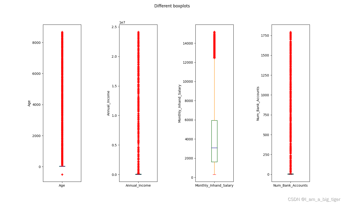

 

 

 

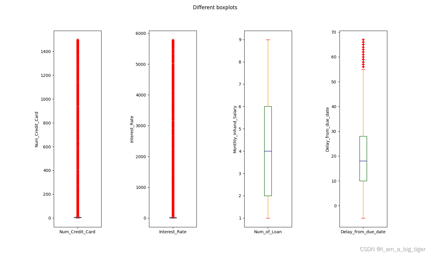
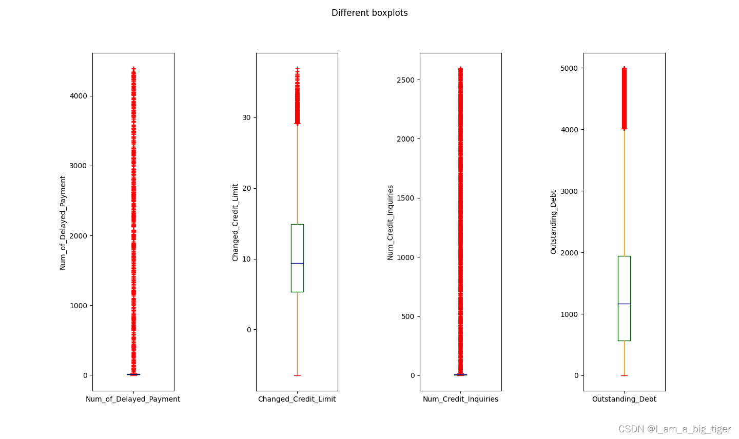
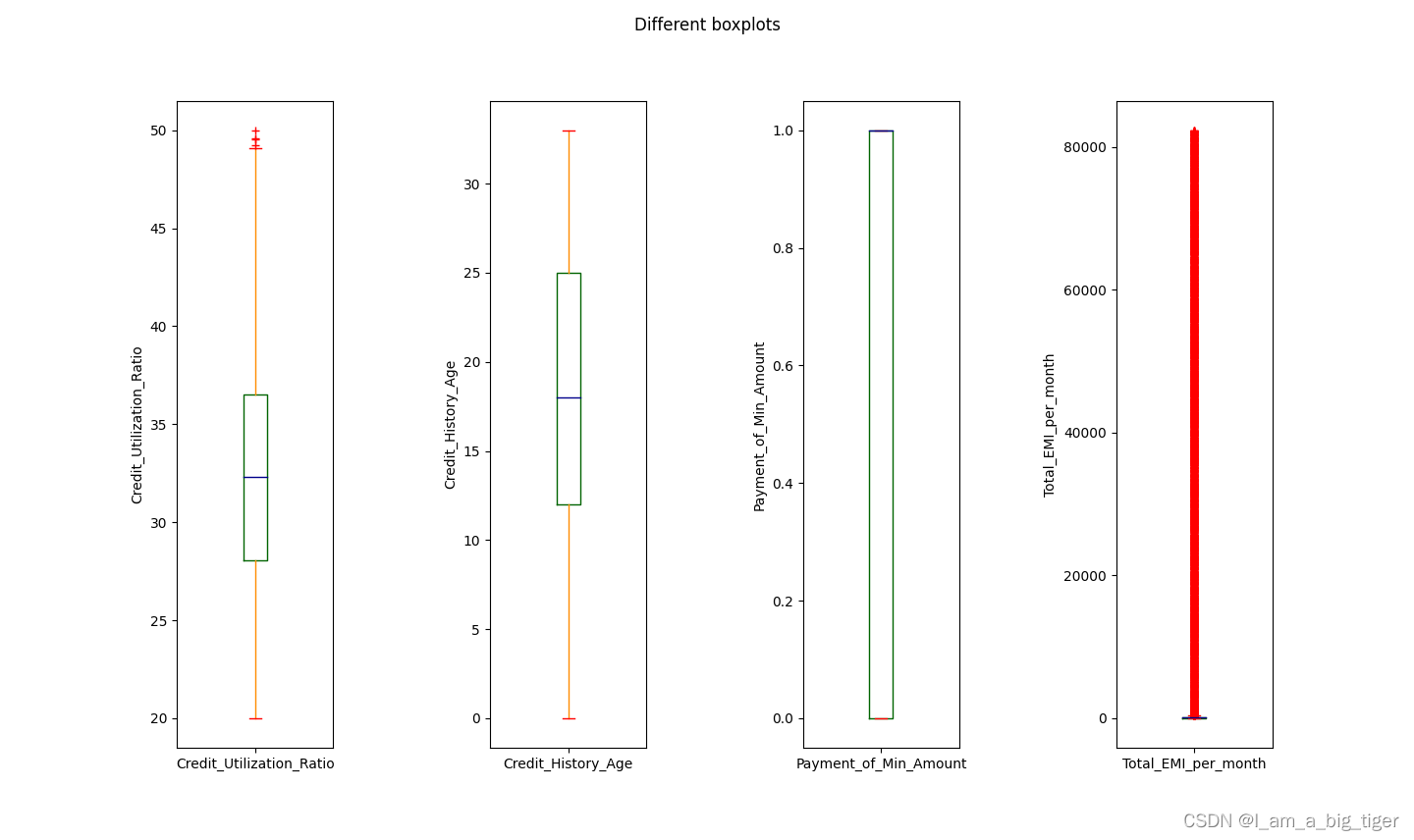
6.根据箱线图分析，对不同特征变量异常值处理采用不同的方式：Age将负值和大于100的值变为空值；综合考虑月收入和年收入，将年收入大于200000变为空值，依次对变量的范围进行设定。之所以变为空值，主要是考虑存在同一个客户（Customer_ID）有多条业务（ID）记录，因此可以使用相同客户id的数据来填充。使用SQL处理异常值。

select case when Age <0 or Age >100 then null  else Age end as Age,
         case when Annual_Income >200000 then null else Annual_Income end as Annual_Income,
         case when Interest_Rate>200 then null else Interest_Rate end as Interest_Rate_1,
         case when Num_Credit_Card>20 then null else Num_Credit_Card end as Num_Credit_Card,
         case when Num_Bank_Accounts<0 or Num_Bank_Accounts> 20 then null else Num_Bank_Accounts
         end as Num_Bank_Accounts_1,
         case when Num_Credit_Inquiries>50 then null else Num_Credit_Inquiries end as Num_Credit_Inquiries
from train；

7.先查看经过上一步处理之后数据的缺失情况。下一步处理思路，Credit_Mix 使用随机森林方法缺失值填充，Age，Monthly_Inhand_Salary,Num_of_Loan ，Credit_History_Age，Amount_invested_monthly ，Num_of_Delayed_Payment，Changed_Credit_Limit , Num_Credit_Inquiries,Monthly_Balance 等等使用同一个客户其他不缺失的值来填充。  

##查看各个特征缺失率
data = pd.read_csv(r"D:\new_job\KAGGLE\kaggle\train_1.csv")
missingDf = df.isnull().sum().sort_values(ascending=False).reset_index()
missingDf.columns = ['feature','missing']
missingDf['per-missing'] = missingDf['missing']/df.shape[0]
print(missingDf)

              feature  missing  per-missing
0                 Credit_Mix    20195      0.20195
1      Monthly_Inhand_Salary    15002      0.15002
2                Num_of_Loan    11408      0.11408
3         Credit_History_Age     9030      0.09030
4    Amount_invested_monthly     8784      0.08784
5     Num_of_Delayed_Payment     7002      0.07002
6       Changed_Credit_Limit     2091      0.02091
7       Num_Credit_Inquiries     1965      0.01965
8            Monthly_Balance     1200      0.01200
9   Credit_Utilization_Ratio        0      0.00000
10         Payment_Behaviour        0      0.00000
11       Total_EMI_per_month        0      0.00000
12     Payment_of_Min_Amount        0      0.00000
13                        ID        0      0.00000
14          Outstanding_Debt        0      0.00000
15               Customer_ID        0      0.00000
16       Delay_from_due_date        0      0.00000
17             Interest_Rate        0      0.00000
18           Num_Credit_Card        0      0.00000
19         Num_Bank_Accounts        0      0.00000
20             Annual_Income        0      0.00000
21                       Age        0      0.00000
22              Credit_Score        0      0.00000

8.异常值补充方法：使用下一条数据补充异常值

'''
----异常值填充:用下一条值填充
Age,Monthly_Inhand_Salary,Num_of_Loan ，Credit_History_Age，Amount_invested_monthly ，
Num_of_Delayed_Payment，Changed_Credit_Limit , Num_Credit_Inquiries,Monthly_Balance 
'''
data['Age'].fillna(method='bfill', inplace=True)
data['Monthly_Inhand_Salary'].fillna(method='bfill', inplace=True)
data['Num_of_Loan'].fillna(0,inplace=True)  # 没有债务的用0填充
data['Credit_History_Age'].fillna(method='bfill', inplace=True)
data['Amount_invested_monthly'].fillna(method='bfill', inplace=True)
data['Num_of_Delayed_Payment'].fillna(method='bfill', inplace=True)
data['Changed_Credit_Limit'].fillna(method='bfill', inplace=True)
data['Num_Credit_Inquiries'].fillna(method='bfill', inplace=True)
data['Monthly_Balance'].fillna(method='bfill', inplace=True)
data['Num_Credit_Card'].fillna(method='bfill', inplace=True)
data['Interest_Rate'].fillna(method='bfill', inplace=True)
data['Num_Bank_Accounts'].fillna(method='bfill', inplace=True)
data['Annual_Income'].fillna(method='bfill', inplace=True)

9.随机森林填充异常值。到此数据基础处理完毕。

'''
Credit_Mix 特征处理:
---用Credit_Mix 特征值非空的样本构建训练集，用缺失的样本构建测试集
'''
from sklearn.ensemble import RandomForestRegressor
data = pd.read_csv(r"D:\new_job\KAGGLE\kaggle\train_2.csv")
rfDf = data.iloc[:,[8,2,3,4,5,6,7,9,10,11,12,13,14,15,16,17,18,19,20,21]]  ##原始数据集中的无缺失数据特征
rfDf_train = rfDf.loc[rfDf['Credit_Mix'].notnull()]
rfDf_test = rfDf.loc[rfDf['Credit_Mix'].isnull()]

##划分训练数据和标签（Label）
X = rfDf_train.iloc[:,1:]
y = rfDf_train.iloc[:,0]
##训练过程
rf = RandomForestRegressor(random_state=0,n_estimators=20,max_depth=3,n_jobs=-1)
rf.fit(X,y)
##预测过程
pred = rf.predict(rfDf_test.iloc[:,1:]).round()
df.loc[(df['Credit_Mix'].isnull()),'Credit_Mix'] = pred
print(df['Credit_Mix'].describe())
data.to_csv(r"D:\new_job\KAGGLE\kaggle\train_3.csv")

二、相关性分析，特征筛选

1.计算皮尔逊相关系数，相关性大于0.6的特征，查看显著性，显著性小于0.05，认为显著。对于相关性大于0.6且关系显著的特征，保留其中区分性好、稳定性强的一个。

'''计算皮尔逊相关系数'''
import matplotlib.pyplot as plt
import seaborn as sns
from scipy.stats import pearsonr

data = pd.read_csv(r"D:\new_job\KAGGLE\kaggle\train_3.csv")
cor = data.columns[3:]
cor = list(cor)
pearson_mat = data[cor].corr(method='pearson')
plt.figure(figsize=(20,15))
sns.heatmap(pearson_mat,square=True,annot=True,cmap='YlGnBu')
plt.show()
'''
查看变量之间的显著性
'''
print(data.columns)
r1,p_value1 = pearsonr(data['Annual_Income'],data['Monthly_Inhand_Salary'])
print(r1,p_value1)  ##0.9744325673262497 0.0
r2,p_value2 = pearsonr(data['Credit_Mix'],data['Outstanding_Debt'])
print(r2,p_value2)
r3,p_value3 = pearsonr(data['Num_of_Loan'],data['Outstanding_Debt'])
print(r3,p_value3)
r4,p_value4 = pearsonr(data['Credit_Mix'],data['Num_of_Loan'])
print(r4,p_value4)
r5,p_value5 = pearsonr(data['Interest_Rate'],data['Outstanding_Debt'])
print(r5,p_value5)
r6,p_value6 = pearsonr(data['Interest_Rate'],data['Credit_Mix'])
print(r6,p_value6)
r7,p_value7 = pearsonr(data['Annual_Income'],data['Amount_invested_monthly'])
print(r7,p_value7)
r8,p_value8 = pearsonr(data['Monthly_Inhand_Salary'],data['Amount_invested_monthly'])
print(r8,p_value8)
r9,p_value9 = pearsonr(data['Credit_Mix'],data['Delay_from_due_date'])
print(r9,p_value9)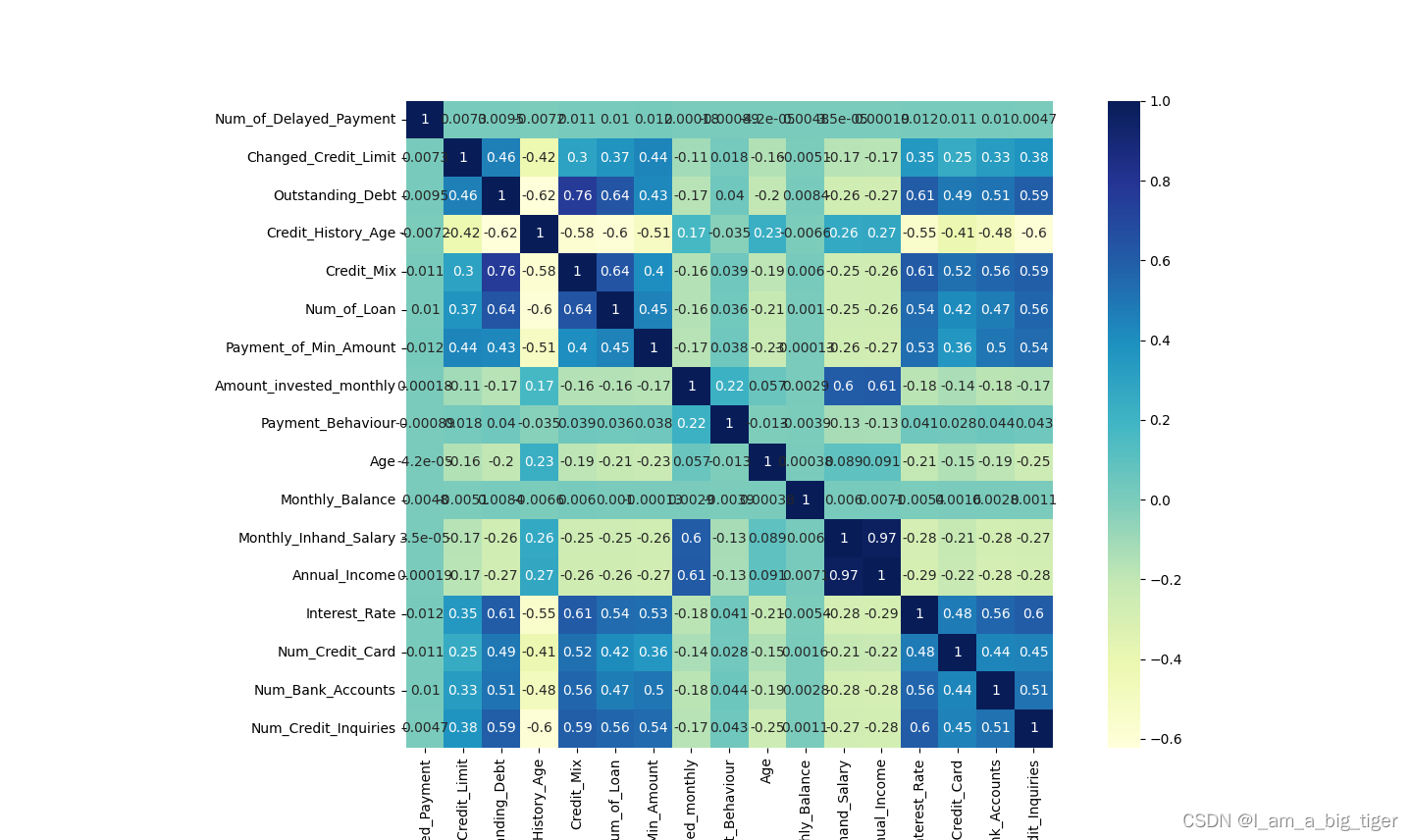

2.查看变量的多重共线性，使用逐步回归法（stepwise regression），筛选并删除引起多重共线性的方法。['Target', 'Credit_Utilization_Ratio', 'Num_of_Delayed_Payment', 'Credit_History_Age', 'Num_of_Loan', 'Age', 'Num_Credit_Card', 'Num_Bank_Accounts']，这些特征被留下。接下来的分析使用这些被保留的数据。

'''
使用逐步回归方法筛选并删除引起多重共线性的变量
'''
import  toad
final_data = toad.selection.stepwise(data,
                                     target=data.Target,
                                     estimator='lr',
                                     direction='both',
                                     criterion='aic',
                                     return_drop=False)
select_cols = final_data.columns
print(select_cols)

三、分箱，woe编码，计算IV值

1.先定义一个分箱函数，先观察各特征分箱情况，查看分箱单调性，找到分箱区间。发现woe都具有较好的单调性，可以采用以上分箱区间。

from scipy import stats  ##导入一个推断包

def optimal_bins(Y,X,n):
    '''
    :param Y: 目标变量
    :param X:待分箱特征
    :param n:分箱数初始值
    :return:统计值，分箱边界值列表，woe，iv
    '''
    r = 0
    total_bad =Y.sum() ##总的坏样本
    total_good = Y.count()-total_bad ##总的好样本
    ##分箱过程
    while np.abs(r)<1:
        df1 = pd.DataFrame({'X':X,'Y':Y,'bin':pd.qcut(X,n,duplicates='drop')})
        df2 = df1.groupby('bin')
        r,p = stats.spearmanr(df2.mean().X,df2.mean().Y)
        n=n-1
    ##计算woe和iv值
    df3 = pd.DataFrame()
    df3['min_'+X.name] = df2.min().X
    df3['max_'+X.name] = df2.max().X
    df3['sum'] = df2.sum().Y
    df3['total'] = df2.count().Y
    df3['rate'] = df2.mean().Y
    df3['badattr'] = df3['sum']/total_bad
    df3['goodattr'] = (df3['total']-df3['sum'])/total_good
    df3['woe'] = np.log(df3['badattr']/df3['goodattr'])
    iv = ((df3['badattr']-df3['goodattr'])*df3['woe']).sum()
    df3 = df3.sort_values(by='min_'+X.name).reset_index(drop=True)
    ##分箱边界值列表
    cut = []
    cut.append(float('-inf'))
    for i in range(1,n+1):
        qua = X.quantile(i/(n+1))
        cut.append(round(qua,6))
    cut.append(float('inf'))
    ##woe值列表
    woe = list(df3['woe'])
    return df3,cut,woe,iv
##观察各特征分箱情况，例如
'Delay_from_due_date'
df_dfdd,cut_dfdd,woe_dfdd,iv_dfdd = optimal_bins(data.Target,data.Delay_from_due_date,n=10)
print(df_dfdd)

min_Delay_from_due_date  max_Delay_from_due_date   sum  total      rate  \
0                       -5                        7  1959  17275  0.113401   
1                        8                       11  1898  13020  0.145776   
2                       12                       15  2173  13474  0.161274   
3                       16                       21  4560  15265  0.298723   
4                       22                       27  4550  14769  0.308078   
5                       28                       38  5021  12434  0.403812   
6                       39                       67  8837  13763  0.642084   

    badattr  goodattr       woe  
0  0.067556  0.215712 -1.160983  
1  0.065453  0.156643 -0.872643  
2  0.074936  0.159165 -0.753301  
3  0.157252  0.150770  0.042093  
4  0.156907  0.143926  0.086360  
5  0.173150  0.104406  0.505875  
6  0.304745  0.069378  1.479901 

2.分箱，woe编码，计算iv值，筛选变量，其他变量iv值大于0.02，Credit_Utilization_Ratio  iv= 0.004521，删除。

'''定义分箱函数'''
def custom_bins(Y,X,binlist):
    '''
    :param Y: 目标变量
    :param X: 待分箱特征
    :param binlist: 分箱边界值列表
    :return: 统计值，woe值，iv值
    '''
    r = 0
    total_bad = Y.sum()  ##总的坏样本
    total_good = Y.count() - total_bad  ##总的好样本
    #等距分箱
    df1 = pd.DataFrame({'X':X,'Y':Y,'bin':pd.cut(X,binlist)})
    df2 = df1.groupby('bin',as_index=True)
    r,p = stats.spearmanr(df2.mean().X,df2.mean().Y)
    df3 = pd.DataFrame()
    df3['min_' + X.name] = df2.min().X
    df3['max_' + X.name] = df2.max().X
    df3['sum'] = df2.sum().Y
    df3['total'] = df2.count().Y
    df3['rate'] = df2.mean().Y
    df3['badattr'] = df3['sum'] / total_bad
    df3['goodattr'] = (df3['total'] - df3['sum']) / total_good
    df3['woe'] = np.log(df3['badattr'] / df3['goodattr'])
    iv = ((df3['badattr'] - df3['goodattr']) * df3['woe']).sum()
    df3 = df3.sort_values(by='min_' + X.name).reset_index(drop=True)
    woe = list(df3['woe'])

    return df3,woe,iv

'''自定义分箱区间如下'''
#原始特征
ninf = float('-inf')
pinf = float('inf')
cut_cur = [ninf, 28.052567, 32.305784, 36.496663, pinf]
cut_ndp = [ninf,6.0, 9.0, 11.0, 14.0, 16.0, 18.0, 21.0,pinf]
cut_cha = [ninf,12.0, 18.0, 25.0,pinf]
cut_nol = [ninf, 2.0, 3.0, 5.0,pinf]
cut_age = [ninf,24.0, 33.0, 42.0,pinf]
cut_ncc = [ninf,4.0, 5.0, 7.0,pinf]
cut_nba = [ninf,3.0, 5.0, 7.0,pinf]


##查看统计值、woe、iv
df_cur,woe_cur,iv_cur = custom_bins(data.Target,data.Credit_Utilization_Ratio,cut_cur)
df_ndp,woe_ndp,iv_ndp = custom_bins(data.Target,data.Num_of_Delayed_Payment,cut_ndp)
df_cha,woe_cha,iv_cha = custom_bins(data.Target,data.Credit_History_Age,cut_cha)
df_nol,woe_nol,iv_nol = custom_bins(data.Target,data.Num_of_Loan,cut_nol)
df_ir,woe_ir,iv_ir = custom_bins(data.Target,data.Interest_Rate,cut_ir)
df_age,woe_age,iv_age = custom_bins(data.Target,data.Age,cut_age)
df_ncc,woe_ncc,iv_ncc = custom_bins(data.Target,data.Num_Credit_Card,cut_ncc)
df_nba,woe_nba,iv_nba = custom_bins(data.Target,data.Num_Bank_Accounts,cut_nba)

'''woe编码'''
data['Credit_Utilization_Ratio'] = pd.cut(data['Credit_Utilization_Ratio'],bins=cut_cur,labels=woe_cur)
data['Num_of_Delayed_Payment'] = pd.cut(data['Num_of_Delayed_Payment'],bins=cut_ndp,labels=woe_ndp)
data['Credit_History_Age'] = pd.cut(data['Credit_History_Age'],bins=cut_cha,labels=woe_cha)
data['Num_of_Loan'] = pd.cut(data['Num_of_Loan'],bins=cut_nol,labels=woe_nol)
data['Age'] = pd.cut(data['Age'],bins=cut_age,labels=woe_age)
data['Num_Credit_Card'] = pd.cut(data['Num_Credit_Card'],bins=cut_ncc,labels=woe_ncc)
data['Num_Bank_Accounts'] = pd.cut(data['Num_Bank_Accounts'],bins=cut_nba,labels=woe_nba)


df = data[['Target','Credit_Utilization_Ratio','Num_of_Delayed_Payment','Credit_History_Age',
           'Num_of_Loan','Age','Num_Credit_Card','Num_Bank_Accounts']]



# df.to_csv(r"D:\new_job\KAGGLE\kaggle\train_4_woe.csv")


'''查看iv列表'''
df = pd.read_csv(r"D:\new_job\KAGGLE\kaggle\train_4_woe.csv")
ivDf = pd.DataFrame(columns=['feature','iv'])
feaList = list(df.columns[1:])
ivList = [iv_cur,iv_ndp,iv_cha,iv_nol,iv_age,iv_ncc,iv_nba]
for i,x in enumerate(feaList):
    ivDf.loc[i,'feature'] = x
    ivDf.loc[i,'iv'] = ivList[i]
ivDf = ivDf.sort_values(by='iv',ascending=False).reset_index(drop=True)
print(ivDf)
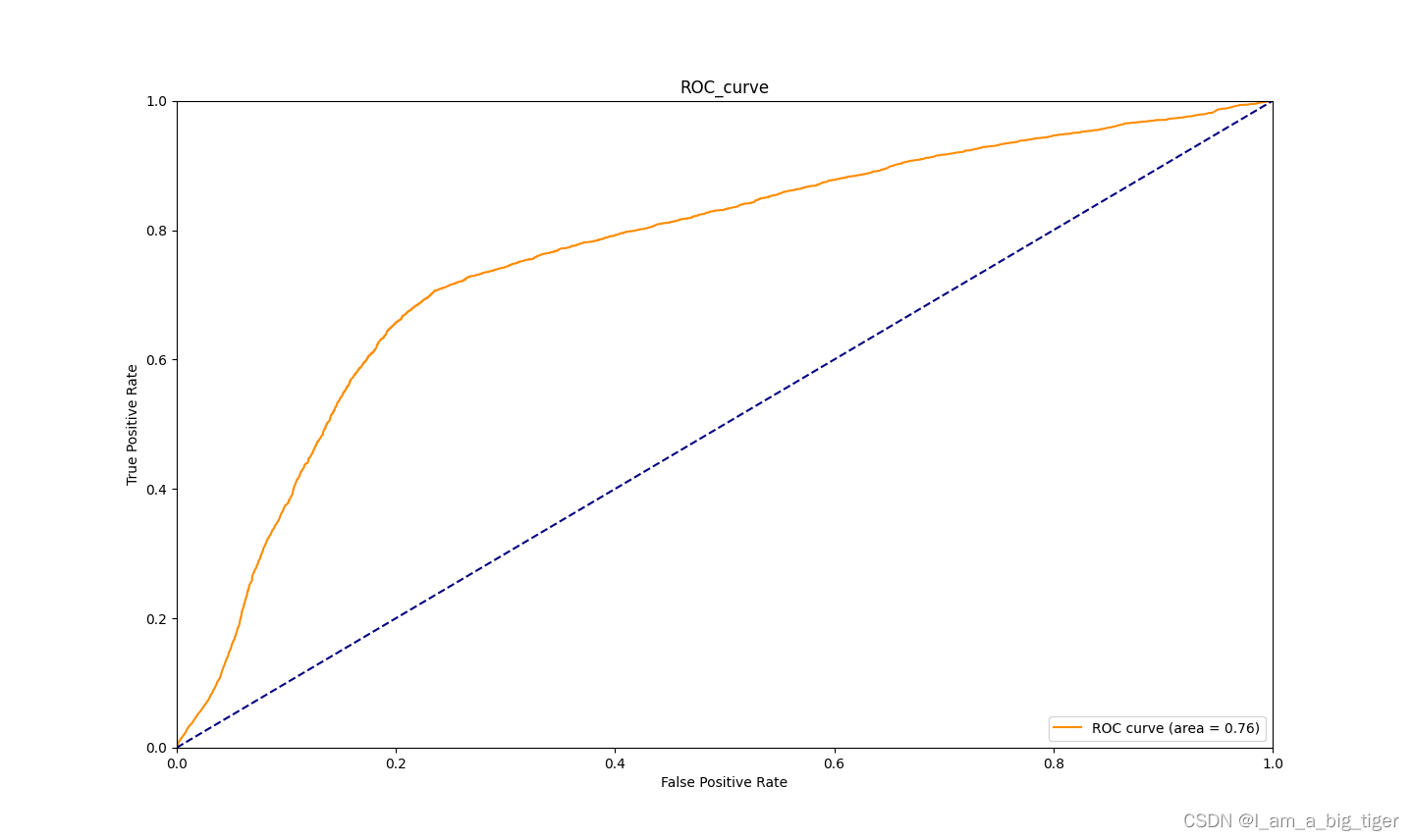
# ivDf.to_csv(r"D:\new_job\KAGGLE\archive\ivDf.csv")

四、变量入模训练，auc=0.76，ks=0.47

from sklearn.linear_model import LogisticRegression
from sklearn.metrics import auc,roc_curve
from sklearn.model_selection import train_test_split
'''
LogisticRegression 一些重要参数的默认值
penalty：正则化类型，默认值'L2',当solver='liblinear'时，还可以选择‘l1’
tol:迭代终止的阈值，默认值为le-4
max_iter：最大迭代次数，默认值为100
'''
'划分训练集和测试集'
df = pd.read_csv(r"D:\new_job\KAGGLE\kaggle\train_4_woe.csv")
X = df.iloc[:,1:]
Y = df.iloc[:,0]
X_train,X_test,Y_train,Y_test = train_test_split(X,Y,test_size=0.3,random_state=0)

'模型训练'
lr = LogisticRegression(random_state=0,solver='liblinear',class_weight={0:0.4,1:0.6},penalty='l1')
k_train = lr.fit(X_train,Y_train)

'模型预测'
Y_pred = k_train.predict(X_test)
Y_score = lr.decision_function(X_test)

'''模型结果评估'''
fpr1,tpr1,threshold = roc_curve(Y_test,Y_score)
auc_value = auc(fpr1,tpr1)

#画图
plt.figure(figsize=(20,15))
plt.plot(fpr1, tpr1, color='darkorange',label='ROC curve (area = %0.2f)' % auc_value)
plt.plot([0, 1], [0, 1], color='navy',  linestyle='--')
plt.xlim([0.0, 1.0])
plt.ylim([0.0, 1.0])
plt.xlabel('False Positive Rate')
plt.ylabel('True Positive Rate')
plt.title('ROC_curve')
plt.legend(loc="lower right")
plt.show()
print('AUC值：',auc_value)

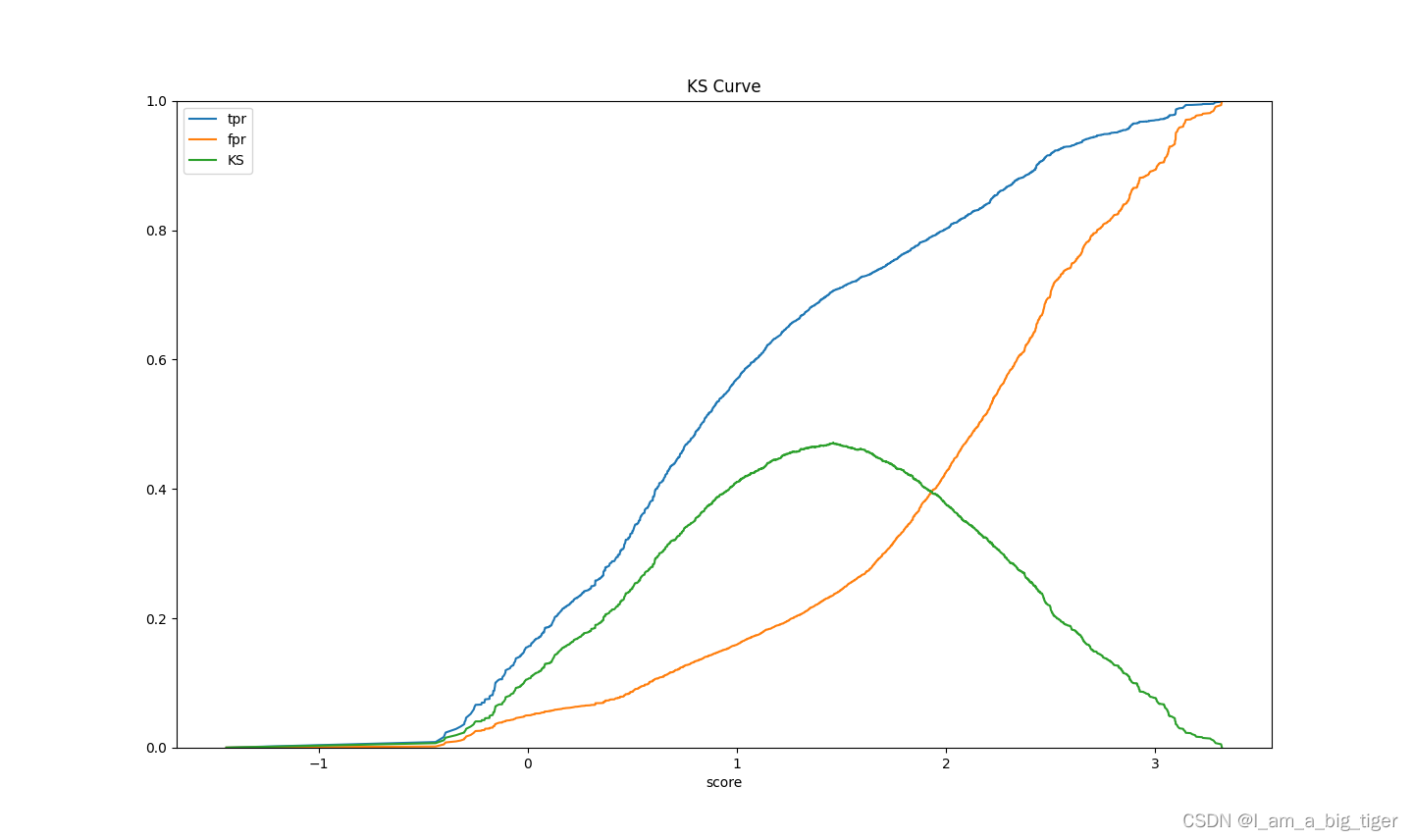
'计算KS值'
fig, ax = plt.subplots()
ax.plot(1 - threshold, tpr1, label='tpr') # ks曲线要按照预测概率降序排列，所以需要1-threshold镜像
ax.plot(1 - threshold, fpr1, label='fpr')
ax.plot(1 - threshold, tpr1-fpr1,label='KS')
#画图
plt.xlabel('score')
plt.title('KS Curve')
plt.ylim([0.0, 1.0])
plt.figure(figsize=(20,20))
legend = ax.legend(loc='upper left')
plt.show()
print('KS值：',max(tpr1-fpr1))

五、模型AUC=0.76、KS=0.47效果。