【KAN】KAN神经网络学习训练营(24)——Example 3：分类

Kolmogorov-Arnold 表示定理Kolmogorov-Arnold 表示定理指出，如果是有界域上的多元连续函数，那么它可以写为单个变量的连续函数的有限组合，以及加法的二进制运算。更具体地说，对于光滑其中和。从某种意义上说，他们表明唯一真正的多元函数是加法，因为所有其他函数都可以使用单变量函数和 sum 来编写。然而，这个 2 层宽度 - Kolmogorov-Arnold 表示可

灵犀拾荒者

1029人浏览 · 2025-04-10 10:00:00

灵犀拾荒者 · 2025-04-10 10:00:00 发布

一、引言

KAN神经网络（Kolmogorov–Arnold Networks）是一种基于Kolmogorov-Arnold表示定理的新型神经网络架构。该定理指出，任何多元连续函数都可以表示为有限个单变量函数的组合。与传统多层感知机（MLP）不同，KAN通过可学习的激活函数和结构化网络设计，在函数逼近效率和可解释性上展现出潜力。

二、技术与原理简介

1.Kolmogorov-Arnold 表示定理

Kolmogorov-Arnold 表示定理指出，如果是有界域上的多元连续函数，那么它可以写为单个变量的连续函数的有限组合，以及加法的二进制运算。更具体地说，对于光滑 $ff:[0,1]^{^{n}}\rightarrow \mathbb{R}$

$f \left( x \right)=f \left( x_{1}, \cdots,x_{n} \right)= \sum_{q=1}^{2n+1} \Phi_{q} \left( \sum_{p=1}^{n} \phi_{q,p} \left( x_{p} \right) \right)$

其中和。从某种意义上说，他们表明唯一真正的多元函数是加法，因为所有其他函数都可以使用单变量函数和 sum 来编写。然而，这个 2 层宽度 - Kolmogorov-Arnold 表示可能不是平滑的由于其表达能力有限。我们通过以下方式增强它的表达能力将其推广到任意深度和宽度。 $\boldsymbol{\phi_{q,p}:[0,1]\to\mathbb{R}}$ ， $\boldsymbol{\Phi_{q}:\mathbb{R}\to\mathbb{R}(2n+1)}$

2.Kolmogorov-Arnold 网络（KAN）

Kolmogorov-Arnold 表示可以写成矩阵形式

$f(x)=\mathbf{\Phi_{out}}\mathsf{o}\mathbf{\Phi_{in}}\mathsf{o}{}x$

其中

$\mathbf{\Phi}_{\mathrm{in}}=\begin{pmatrix}\phi_{1,1}(\cdot)&\cdots&\phi_{1,n }(\cdot)\\ \vdots&&\vdots\\ \phi_{2n+1,1}(\cdot)&\cdots&\phi_{2n+1,n}(\cdot)\end{pmatrix}$

$\quad\mathbf{ \Phi}_{\mathrm{out}}=\left(\Phi_{1}(\cdot)\quad\cdots\quad\Phi_{2n+1}(\cdot)\right)$

我们注意到和都是以下函数矩阵（包含输入和输出）的特例，我们称之为 Kolmogorov-Arnold 层： $\mathbf{\Phi_{in}} \mathbf{\Phi_{out}} \mathbf{\Phi_{n_{in}n_{out}}}$

其中 $\boldsymbol{n_{\text{in}}=n,n_{\text{out}}=2n+1\Phi_{\text{out}}n_{\text{in}}=2n+1,n_{\text{out}}=1}$ 。

定义层后，我们可以构造一个 Kolmogorov-Arnold 网络只需堆叠层！假设我们有层，层的形状为。那么整个网络是 $Ll^{th} \Phi_{l} \left( n_{l+1},n_{l} \right)$

$\mathbf{KAN(x)}=\mathbf{\Phi_{L-1}}\circ\cdots\circ\mathbf{\Phi_{1}}\circ \mathbf{\Phi_{0}}\circ\mathbf{x}$

相反，多层感知器由线性层和非线错： $\mathbf{W}_{l^{\sigma}}$

$\text{MLP}(\mathbf{x})=\mathbf{W}_{\textit{L-1}}\circ\sigma\circ\cdots\circ \mathbf{W}_{1}\circ\sigma\circ\mathbf{W}_{0}\circ\mathbf{x}$

KAN 可以很容易地可视化。（1） KAN 只是 KAN 层的堆栈。（2）每个 KAN 层都可以可视化为一个全连接层，每个边缘上都有一个1D 函数。

三、代码详解

1. 首先将问题视为回归问题（输出维度=1，MSE损失）

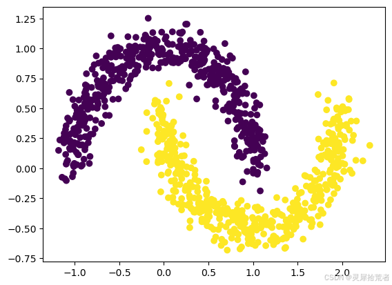
2. 创建双月数据集

from kan import KAN
import matplotlib.pyplot as plt
from sklearn.datasets import make_moons
import torch
import numpy as np

dataset = {}
train_input, train_label = make_moons(n_samples=1000, shuffle=True, noise=0.1, random_state=None)
test_input, test_label = make_moons(n_samples=1000, shuffle=True, noise=0.1, random_state=None)

dataset['train_input'] = torch.from_numpy(train_input)
dataset['test_input'] = torch.from_numpy(test_input)
dataset['train_label'] = torch.from_numpy(train_label[:,None])
dataset['test_label'] = torch.from_numpy(test_label[:,None])

X = dataset['train_input']
y = dataset['train_label']
plt.scatter(X[:,0], X[:,1], c=y[:,0])

3. 训练KAN模型

model = KAN(width=[2,1], grid=3, k=3)

def train_acc():
    return torch.mean((torch.round(model(dataset['train_input'])[:,0]) == dataset['train_label'][:,0]).float())

def test_acc():
    return torch.mean((torch.round(model(dataset['test_input'])[:,0]) == dataset['test_label'][:,0]).float())

results = model.train(dataset, opt="LBFGS", steps=20, metrics=(train_acc, test_acc));
results['train_acc'][-1], results['test_acc'][-1]

4. 自动符号回归

lib = ['x','x^2','x^3','x^4','exp','log','sqrt','tanh','sin','tan','abs']
model.auto_symbolic(lib=lib)
formula = model.symbolic_formula()[0][0]
formula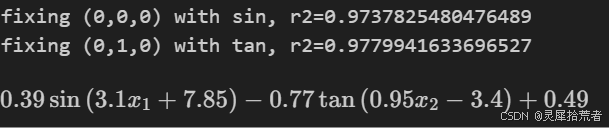

5. 这个公式有多准确？

# how accurate is this formula?
def acc(formula, X, y):
    batch = X.shape[0]
    correct = 0
    for i in range(batch):
        correct += np.round(np.array(formula.subs('x_1', X[i,0]).subs('x_2', X[i,1])).astype(np.float64)) == y[i,0]
    return correct/batch

print('train acc of the formula:', acc(formula, dataset['train_input'], dataset['train_label']))
print('test acc of the formula:', acc(formula, dataset['test_input'], dataset['test_label']))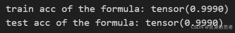

6. 然后将问题视为分类问题（输出维度=2，交叉熵损失）

7. 创建双月数据集

from kan import KAN
import matplotlib.pyplot as plt
from sklearn.datasets import make_moons
import torch
import numpy as np

dataset = {}
train_input, train_label = make_moons(n_samples=1000, shuffle=True, noise=0.1, random_state=None)
test_input, test_label = make_moons(n_samples=1000, shuffle=True, noise=0.1, random_state=None)

dataset['train_input'] = torch.from_numpy(train_input)
dataset['test_input'] = torch.from_numpy(test_input)
dataset['train_label'] = torch.from_numpy(train_label)
dataset['test_label'] = torch.from_numpy(test_label)

X = dataset['train_input']
y = dataset['train_label']
plt.scatter(X[:,0], X[:,1], c=y[:])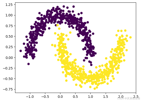

8. 训练KAN模型

model = KAN(width=[2,2], grid=3, k=3)

def train_acc():
    return torch.mean((torch.argmax(model(dataset['train_input']), dim=1) == dataset['train_label']).float())

def test_acc():
    return torch.mean((torch.argmax(model(dataset['test_input']), dim=1) == dataset['test_label']).float())

results = model.train(dataset, opt="LBFGS", steps=20, metrics=(train_acc, test_acc), loss_fn=torch.nn.CrossEntropyLoss());

9. 自动符号回归

lib = ['x','x^2','x^3','x^4','exp','log','sqrt','tanh','sin','abs']
model.auto_symbolic(lib=lib)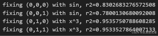

formula1, formula2 = model.symbolic_formula()[0]
formula1

formula2

10. 这个公式有多准确？

# how accurate is this formula?
def acc(formula1, formula2, X, y):
    batch = X.shape[0]
    correct = 0
    for i in range(batch):
        logit1 = np.array(formula1.subs('x_1', X[i,0]).subs('x_2', X[i,1])).astype(np.float64)
        logit2 = np.array(formula2.subs('x_1', X[i,0]).subs('x_2', X[i,1])).astype(np.float64)
        correct += (logit2 > logit1) == y[i]
    return correct/batch

print('train acc of the formula:', acc(formula1, formula2, dataset['train_input'], dataset['train_label']))
print('test acc of the formula:', acc(formula1, formula2, dataset['test_input'], dataset['test_label']))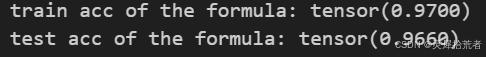

四、总结与思考

KAN神经网络通过融合数学定理与深度学习，为科学计算和可解释AI提供了新思路。尽管在高维应用中仍需突破，但其在低维复杂函数建模上的潜力值得关注。未来可能通过改进计算效率、扩展理论边界，成为MLP的重要补充。

1. KAN网络架构

关键设计：可学习的激活函数：每个网络连接的“权重”被替换为单变量函数（如样条、多项式），而非固定激活函数（如ReLU）。分层结构：输入层和隐藏层之间、隐藏层与输出层之间均通过单变量函数连接，形成多层叠加。参数效率：由于理论保证，KAN可能用更少的参数达到与MLP相当或更好的逼近效果。
示例结构：输入层 → 隐藏层：每个输入节点通过单变量函数 $\phi_{q,i} \left( x_{i} \right)$ 连接到隐藏节点。隐藏层 → 输出层：隐藏节点通过另一组单变量函数 $\psi_{q}$ 组合得到输出。

2. 优势与特点

高逼近效率：基于数学定理，理论上能以更少参数逼近复杂函数；在低维科学计算任务（如微分方程求解）中表现优异。
可解释性：单变量函数可可视化，便于分析输入变量与输出的关系；网络结构直接对应函数分解过程，逻辑清晰。
灵活的函数学习：激活函数可自适应调整（如学习平滑或非平滑函数）；支持符号公式提取（例如从数据中恢复物理定律）。

3. 挑战与局限

计算复杂度：单变量函数的学习（如样条参数化）可能增加训练时间和内存消耗。需要优化高阶连续函数，对硬件和算法提出更高要求。
泛化能力：在高维数据（如图像、文本）中的表现尚未充分验证，可能逊色于传统MLP。
训练难度：需设计新的优化策略，避免单变量函数的过拟合或欠拟合。

4. 应用场景

科学计算：求解微分方程、物理建模、化学模拟等需要高精度函数逼近的任务。
可解释性需求领域：医疗诊断、金融风控等需明确输入输出关系的场景。
符号回归：从数据中自动发现数学公式（如物理定律）。

5. 与传统MLP的对比

6. 研究进展

近期论文：2024年，MIT等团队提出KAN架构（如论文《KAN: Kolmogorov-Arnold Networks》），在低维任务中验证了其高效性和可解释性。
开源实现：已有PyTorch等框架的初步实现。

【作者声明】

本文分享的论文内容及观点均来源于《KAN: Kolmogorov-Arnold Networks》原文，旨在介绍和探讨该研究的创新成果和应用价值。作者尊重并遵循学术规范，确保内容的准确性和客观性。如有任何疑问或需要进一步的信息，请参考论文原文或联系相关作者。

【关注我们】

如果您对神经网络、群智能算法及人工智能技术感兴趣，请关注【灵犀拾荒者】，获取更多前沿技术文章、实战案例及技术分享！

技术共进，成长同行——讯飞AI开发者社区

更多推荐

论文笔记：AlphaEdit: Null-Space Constrained Knowledge Editing for Language Models（AlphaEdit）

论文发表于人工智能顶会ICLR（基于定位和修改的模型编辑方法（针对和等）会破坏LLM中最初保存的知识，特别是在顺序编辑场景。为此，本文提出AlphaEdit：1、在将保留知识应用于参数之前，将扰动投影到保留知识的零空间上。2、从理论上证明，这种预测确保了在查询保留的知识时，编辑后的LLM的输出保持不变，从而减轻中断问题。3、对各种LLM（包括LLaMA3、GPT2XL和GPT-J）的广泛实验表明，