提示：可以结合西瓜书等资源进行观看理解

---

前言

随着人工智能的不断发展，机器学习这门技术也越来越重要，很多人都开启了学习机器学习，本文就介绍了机器学习的基础内容。

一、理论部分

章节一：初识人工智能

E experience

P performance

T task

目的是为了提高在T上的P，经过E之后P会得到提高。

学习算法：
最主要的两类：监督学习（supervised learning）、无监督学习（unsupervised learning）

监督学习：

我们给算法一个数据集，其中包含了正确的答案，算法的目的是给出更多的正确答案。

回归问题：回归即我们设法预测连续值的属性（个人理解：数据拟合）

分类问题：预测一个离散值的属性

无监督学习：
没有任何标签或都具有相同的标签，给你大量的数据，要求找出数据中的数据结构

聚类算法：簇（cluster）

鸡尾酒算法：可以将叠加的声音拆开

【W,s,v】=svd((repment(sum(x.*x,1),size(x,1),1).*x)*x’);

Octave软件

章节二：单变量线性回归

 线性模型

符号：
m：训练样本的数量

X：代表输入变量

Y：代表输出变量

（x，y）表示一个训练样本

带上上标表示特定的一条训练样本

模型训练流程：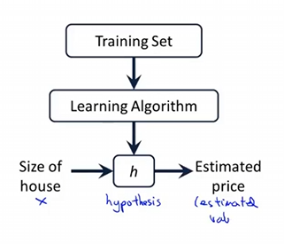

线性回归模型

单变量线性回归

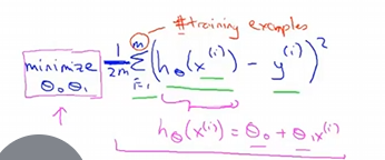
我们想要线性拟合出一个函数，需要求其中的参数，为了求其中的参数，我们提出了cost function，也就是代价函数

代价函数：
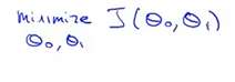
最小化问题：尽量减少假设的输出与房子的真实价格的差值的平方

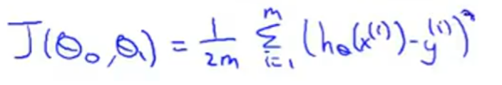
线性回归的整体目标函数（代价函数，平方误差函数）：

梯度下降算法:

A:=b 赋值运算

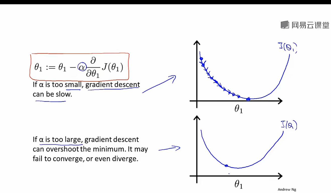
学习率：用来控制步子迈多大

学习率太小会导致的情况：

梯度下降的速率太慢了
学习率太大会导致的情况：

会导致无法收敛甚至发散

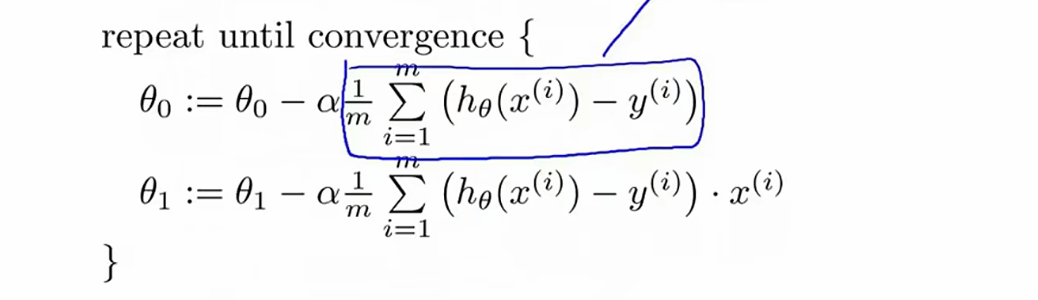
为什么参数要实现同步更新？

参数必须同步更新的根本原因是，为了确保梯度下降是在当前点的“真实梯度”方向上进行搜索和移动。

直白一点的说法就是：对于一个固定的参数，另一个参数会找到最小的损失函数，但是并不是两个整体最小的，虽然我在这个点的这个参数是最小的，但并不是所有的参数的损失函数最小的。

线性回归算法

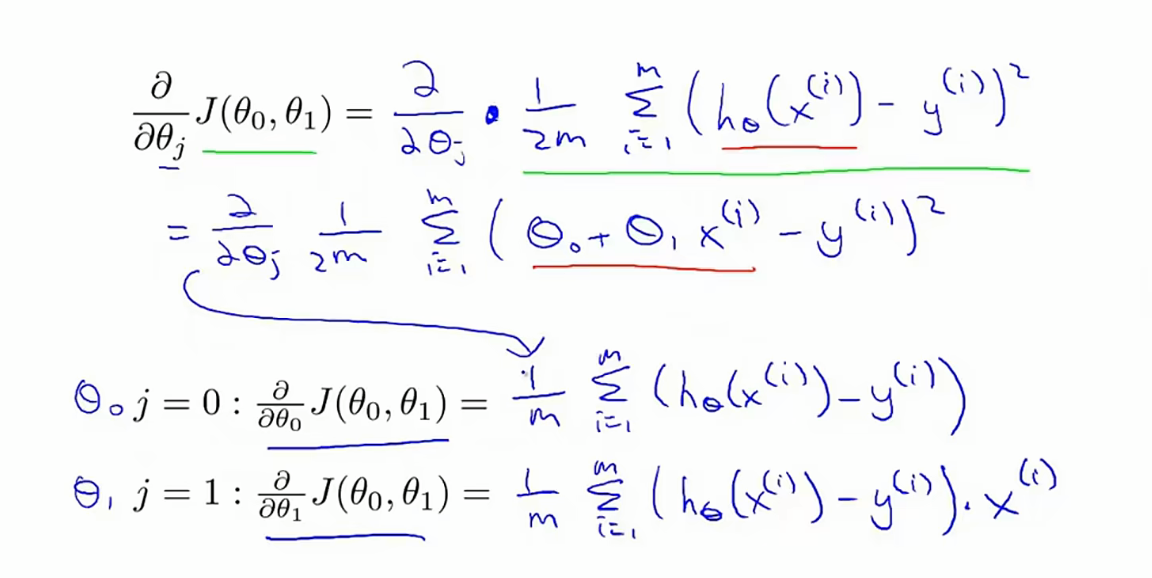
将算出的结果带回到梯度下降算法中得到

对于线性回归函数来说没有局部最优解，只有全局最优解

正规方程组解法，但梯度下降更适用于大数据

二、代码实操

import numpy as np
import matplotlib.pyplot as plt
from mpl_toolkits.mplot3d import Axes3D


# 从文件读取数据
def load_data(filename):
    data = np.loadtxt(filename)
    x = data[:, 0]  # 第一列作为x
    y = data[:, 1]  # 第二列作为y
    return x, y


# 计算误差均方函数 J(w,b)
def  cost_function(x, y, w, b):
    m = x.shape[0]  # 训练集的数据样本数
    cost_sum = 0.0
    for i in range(m):
        f_wb = w * x[i] + b
        cost = (f_wb - y[i]) ** 2
        cost_sum += cost
    return cost_sum / (2 * m)


# 计算梯度值 dJ/dw, dJ/db
def compute_gradient(x, y, w, b):
    m = x.shape[0]  # 训练集的数据样本数
    d_w = 0.0
    d_b = 0.0
    for i in range(m):
        f_wb = w * x[i] + b
        d_wi = (f_wb - y[i]) * x[i]
        d_bi = (f_wb - y[i])
        d_w += d_wi
        d_b += d_bi
    dj_dw = d_w / m
    dj_db = d_b / m
    return dj_dw, dj_db


# 梯度下降算法
def linear_regression(x, y, w, b, learning_rate=0.01, epochs=1000):
    J_history = []  # 记录每次迭代产生的误差值
    for epoch in range(epochs):
        dj_dw, dj_db = compute_gradient(x, y, w, b)
        # w 和 b 需同步更新
        w = w - learning_rate * dj_dw
        b = b - learning_rate * dj_db
        J_history.append(cost_function(x, y, w, b))  # 记录每次迭代产生的误差值
    return w, b, J_history


# 绘制线性方程的图像
def draw_line(w, b, xmin, xmax, title):
    x = np.linspace(xmin, xmax, 100)
    y_pred = w * x + b
    plt.xlabel("X-axis", size=15)
    plt.ylabel("Y-axis", size=15)
    plt.title(title, size=20)
    plt.plot(x, y_pred, 'r-', linewidth=2)


# 绘制散点图
def draw_scatter(x, y, title):
    plt.xlabel("X-axis", size=15)
    plt.ylabel("Y-axis", size=15)
    plt.title(title, size=20)
    plt.scatter(x, y, c='blue', alpha=0.7)


# 绘制3D代价函数曲面图
def plot_3d_cost_surface(x_data, y_data, w_range=(-10, 10), b_range=(-10, 10)):
    # 创建网格
    w_values = np.linspace(w_range[0], w_range[1], 100)
    b_values = np.linspace(b_range[0], b_range[1], 100)
    W, B = np.meshgrid(w_values, b_values)

    # 计算每个(w,b)组合的代价
    J = np.zeros_like(W)
    for i in range(W.shape[0]):
        for j in range(W.shape[1]):
            J[i, j] = cost_function(x_data, y_data, W[i, j], B[i, j])

    # 创建3D图
    fig = plt.figure(figsize=(12, 8))
    ax = fig.add_subplot(111, projection='3d')

    # 绘制曲面
    surf = ax.plot_surface(W, B, J, cmap='viridis', alpha=0.8)
    #  alpha透明度设置

    ax.set_xlabel('Weight (w)', fontsize=12)
    ax.set_ylabel('Bias (b)', fontsize=12)
    ax.set_zlabel('Cost J(w,b)', fontsize=12)
    ax.set_title('3D Cost Function Surface', fontsize=16)

    # 添加颜色条
    fig.colorbar(surf, ax=ax, shrink=0.5, aspect=20)

    return fig, ax


# 绘制等高线图
def plot_contour(x_data, y_data, w_range=(-10, 10), b_range=(-10, 10)):
    # 创建网格
    w_values = np.linspace(w_range[0], w_range[1], 100)
    b_values = np.linspace(b_range[0], b_range[1], 100)
    W, B = np.meshgrid(w_values, b_values)

    # 计算每个(w,b)组合的代价
    J = np.zeros_like(W)
    for i in range(W.shape[0]):
        for j in range(W.shape[1]):
            J[i, j] = cost_function(x_data, y_data, W[i, j], B[i, j])

    # 创建等高线图
    plt.figure(figsize=(10, 8))

    # 绘制等高线
    contour = plt.contour(W, B, J, 50, cmap='viridis')
    plt.clabel(contour, inline=True, fontsize=8)

    plt.xlabel('Weight (w)', fontsize=12)
    plt.ylabel('Bias (b)', fontsize=12)
    plt.title('Cost Function Contour Plot', fontsize=16)
    plt.colorbar(contour, label='Cost J(w,b)')

    return plt.gcf()


# 从这里开始执行
if __name__ == '__main__':
    # 从文件读取数据
    x_train, y_train = load_data('one_variable.txt')
    print(f"成功加载数据: {len(x_train)} 个样本")
    print(f"x数据范围: {x_train.min():.2f} - {x_train.max():.2f}")
    print(f"y数据范围: {y_train.min():.2f} - {y_train.max():.2f}")
    # 初始化参数
    w = 0.0  # 权重
    b = 0.0  # 偏置
    epochs = 10000  # 迭代次数
    learning_rate = 0.01  # 学习率

    # 运行梯度下降
    w, b, J_history = linear_regression(x_train, y_train, w, b, learning_rate, epochs)
    print(f"优化结果: w = {w:.4f}, b = {b:.4f}")
    print(f"最终代价: {J_history[-1]:.6f}")

    # 绘制迭代计算得到的线性回归方程
    plt.figure(1, figsize=(10, 6))
    draw_scatter(x_train, y_train, "Training Data with Regression Line")
    draw_line(w, b, x_train.min() - 1, x_train.max() + 1, f"Linear Regression: y = {w:.2f}x + {b:.2f}")
    plt.grid(True, alpha=0.3)
    plt.legend(['Regression Line', 'Training Data'])
    plt.show()

    # 绘制误差值的收敛曲线
    plt.figure(2, figsize=(10, 6))
    plt.plot(range(epochs), J_history, 'b-', linewidth=1)
    plt.xlabel('Epochs', size=15)
    plt.ylabel('Cost', size=15)
    plt.title('Cost Function Convergence', size=20)
    plt.grid(True, alpha=0.3)
    plt.yscale('log')  # 使用对数坐标更好地显示收敛
    plt.show()

    # 绘制3D代价函数曲面图
    # 根据数据范围调整显示范围
    w_center = w
    b_center = b
    w_range = (w_center - 5, w_center + 5)
    b_range = (b_center - 5, b_center + 5)

    plot_3d_cost_surface(x_train, y_train, w_range, b_range)
    plt.show()

    # 绘制等高线图
    plot_contour(x_train, y_train, w_range, b_range)
    plt.scatter([w], [b], c='red', s=100, marker='x', label='Optimal Point')
    plt.legend()
    plt.show()